The Cost of Ignoring Mode Correlations in Black-Hole
Quasinormal-Mode Resolvability Forecasts

Abstract

Forecasts in black-hole spectroscopy decide whether two quasinormal modes are distinguishable using a Rayleigh-type criterion: the modes are declared resolvable when their frequency and damping-time separations exceed the statistical uncertainties of the corresponding estimates. Those uncertainties can be drawn from the joint two-mode Fisher matrix that keeps the correlations between the mode templates, as the forecast literature does, or from a single-mode analysis that treats each mode as if alone, a natural shortcut when correlations are presumed small. This paper quantifies what the shortcut costs. The ratio between the two resulting signal-to-noise thresholds is computed for damped-sinusoid fits over a finite analysis window, across the full astrophysical spin range and a wide family of window choices, under white noise. For the contested fundamental-overtone pair the correlation-aware threshold exceeds the single-mode one by a factor of about four to eight everywhere on the map (median over relative phase): at remnant spin 0.69 the thresholds are 71 against 310. For a well-separated control pair the factor stays near or below two. The penalty is set almost entirely by the threefold difference in damping times, not by the two-percent frequency splitting, and the template overlap behind it has a simple closed form. Two properties are exact: the ratio is independent of the mode amplitude ratio, and the overlap is invariant under translation of the analysis window, which also removes any remnant-mass dependence under white noise. Individual-phase thresholds spread by tens of percent about the reported medians, and the noise model is white throughout; both limitations are stated where they enter. The full pipeline reproduces every figure with one command.

I Introduction

After two black holes merge, the remnant settles down by emitting gravitational waves at a discrete set of complex frequencies, the quasinormal modes (QNMs) of the final Kerr black hole. Because general relativity fixes every QNM frequency by the remnant’s mass and spin alone, detecting two or more modes in the ringdown and checking their consistency is a direct test of the no-hair theorem, the statement that an isolated black hole carries no structure beyond those two numbers [1, 2]. Whether current detectors have already achieved this with the first overtone of GW150914 (a shorter-lived mode sharing the fundamental’s angular harmonic at nearly the same frequency) remains actively disputed [2, 3].

Forecasts of when such tests become possible rest on a resolvability criterion. The standard choice is Rayleigh-like [1, 4, 5]: two modes are declared distinguishable at a given signal-to-noise ratio (SNR) if their frequency separation exceeds the statistical uncertainty of the frequency estimates, and likewise for the damping times. Its users are not naive about it: Ota and Chirenti found it overly restrictive relative to a Bayes-factor threshold and argued for the latter [4]. The criterion nonetheless continues to anchor quantitative statements throughout the forecast literature [5, 6].

In parallel, the pseudospectrum programme (which maps an operator’s approximate eigenvalues to ask how far its spectrum moves under small perturbations) has put a structural fact on firm footing: the operator governing black-hole ringdown is non-self-adjoint, meaning it differs from its adjoint and so need not admit an orthogonal eigenbasis; its spectrum can be unstable under small perturbations; and its eigenfunctions, the QNMs, are not orthogonal in physically motivated inner products [7, 8, 9]. Estimation theory is unambiguous about what non-orthogonality does to a joint fit: the covariance of the estimated parameters is governed by the correlations of the template set, so the achievable precision is controlled by the conditioning of the template Gram matrix, not by frequency separation alone.

The forecast literature is not naive about these correlations. Berti, Cardoso, and Will, who introduced the criterion in the form used here, already computed its thresholds from a joint two-mode Fisher matrix, naming the “cross-terms” in the inner products as the reason the same-harmonic overtone case resists closed-form treatment [Sec. VII of [1]]; Ota and Chirenti evaluate an eight-parameter joint matrix [Eq. (9) of [4]], and Shi, Zhang, and Mei a twenty-six parameter one [5]. What none of these works isolates is how much of the resulting threshold is the correlation penalty itself: the factor separating the joint-Fisher threshold from a single-mode baseline in which each mode is analyzed as if alone. That baseline is a diagnostic, not a position held in the literature: the two constructions coincide exactly for orthogonal templates, so their ratio directly measures what mode overlap costs the criterion, and to the authors’ knowledge that ratio has not been mapped for the astrophysically contested pairs. This paper computes the map. The working hypothesis (H1) was that the ratio exceeds two somewhere in parameter space, largest for the $(2,2,0)\text{–}(2,2,1)$ fundamental–overtone pair, the same pair contested in GW150914 [2, 3]. The computation returns the strong form of H1: the factor is between 4.25 and 8.1 everywhere on the map (median over relative phase), and near or below 2 for a control pair.

The contributions are:

• both threshold constructions stated in one Fisher framework, pinned to the anchor forecasts’ equations (Section III);

• a map of the correlation penalty over remnant spin and analysis-window start, per mode pair (Section V);

• a closed form for the template overlap that sets the penalty’s scale, showing it is governed by the damping-time ratio rather than the frequency splitting, plus exact invariances with one-line proofs (Sections III-B and VI);

• a reproducible pipeline (laptop-scale; the full map runs in about six minutes; Section IV).

Scope is deliberately narrow. This paper analyzes no detector data, performs no Bayesian inference, and takes no position on whether GW150914’s overtone was real; it audits a criterion, not an event. The inner product is white-noise throughout; detector-shaped weighting and exact reproduction of the anchors’ published horizon numbers are the next milestones and are not claimed here.

II Signal Model and Estimation Framework

II-A Ringdown model

The observed ringdown is modeled over a finite analysis window $t\in [t_0,t_0+T]$ as a sum of damped sinusoids referenced to the waveform peak at $t=0$,

$$h(t)=\sum _k{A}_k{e}^{-t/{\tau }_k}\cos \left(2\pi f_{k}t+{\varphi }_k\right),$$ (1)

where $k$ runs over the mode pair under test and $R=A_1/A_0$ is the amplitude ratio at the peak. The frequencies and damping times are those of the Kerr QNMs,

$$2\pi f_k-\frac{i}{{\tau }_k}=\frac{{\widehat{\omega }}_{\mathrm{\ell }mn}(\chi )}{M_{\mathrm{s}}},M_{\mathrm{s}}\equiv \frac{GM}{c^3},$$ (2)

with ${\widehat{\omega }}_{\mathrm{\ell }mn}(\chi )$ the dimensionless Kerr QNM frequency at spin $\chi$, obtained by table lookup from the qnm package [10]; no QNM frequencies are computed in this work. Here $(\mathrm{\ell },m)$ label the angular harmonic of the perturbation and $n$ is the overtone index, which orders the modes of a given $(\mathrm{\ell },m)$ by decreasing damping time: $n=0$ is the fundamental and $n=1$ its first overtone, the shorter-lived mode at nearly the same frequency. The dimensionless spin is $\chi =cJ/(G{M}^2)\in [0,1)$ for remnant angular momentum $J$, and the map axes run over it. Time dependence is $e^{-i\omega t}$ throughout, so $\mathrm{Re}\widehat{\omega }>0$ and ; the code takes $f=\mathrm{Re}\widehat{\omega }/2\pi$ and $\tau =-1/\mathrm{Im}\widehat{\omega }$ in units of $M$. At $\chi =0.69$ the pair of interest has ${\widehat{f}}_{220}=0.0841$, ${\widehat{\tau }}_{220}=12.3M$ and ${\widehat{f}}_{221}=0.0822$, ${\widehat{\tau }}_{221}=4.07M$: a frequency splitting of only $2.2\%$ against damping times differing by a factor of three.

II-B Inner product, SNR, and Fisher matrix

For white noise of one-sided power spectral density $S_0$, the noise-weighted inner product over the window is

$$⟨a|b⟩=\frac{2}{S_0}{\int }_{t_0}^{t_0+T}a(t)b(t)𝑑t,$$ (3)

and the total SNR is ${\rho }^2=⟨h|h⟩$. With time measured in units of $M$, every quantity entering the analysis is dimensionless, so the results below are exactly independent of the remnant mass; the map axes are spin and window start in units of $M$.

For parameters $\theta =\{A_k,{\varphi }_k,f_k,{\tau }_k\}$, the Fisher matrix and the Cramér–Rao bound on any unbiased estimator are

$${\mathrm{\Gamma }}_{ij}=⟨{\partial }_{i}h|{\partial }_{j}h⟩,{\sigma }_{{\theta }_i}\ge \sqrt{{({\mathrm{\Gamma }}^{-1})}_{ii}}.$$ (4)

All statistical uncertainties below are Fisher-level; this matches the anchor forecasts and is the regime where the Rayleigh criterion is stated.

III Two Constructions of One Criterion

III-A The Rayleigh criterion

Following Berti, Cardoso, and Will [Eqs. (57)–(59) of [1]], as adopted by Ota and Chirenti [Eqs. (6a)–(6b) of [4]], the pair is resolvable at SNR $\rho$ when both separations clear the larger of the corresponding uncertainties,

$$|f_1-f_0|>\max ({\sigma }_{f_0},{\sigma }_{f_1})\text{and}|{\tau }_1-{\tau }_0|>\max ({\sigma }_{{\tau }_0},{\sigma }_{{\tau }_1}).$$ (5)

Every $\sigma$ scales as $1/\rho$ at fixed signal shape, so Eq. 5 defines a critical SNR: the smallest $\rho$ at which both conditions hold. The two constructions differ only in the Fisher matrix that supplies the $\sigma$’s:

• single-mode baseline, critical SNR ${\rho }_{\mathrm{R}}$: each mode’s $(A,\varphi ,f,\tau )$ errors from its own $4\times 4$ Fisher matrix, the other mode absent: the correlation-free reference point, not a procedure attributed to any cited forecast;

• correlation-aware, critical SNR ${\rho }_{\mathrm{C}}$: all errors from the joint $8\times 8$ Fisher matrix of Eq. 1, as the anchor forecasts implement [Eq. (9) of [4]].

The quantity mapped here is the ratio

$$D(\chi ,t_0;\text{pair})={\rho }_{\mathrm{C}}/{\rho }_{\mathrm{R}}\ge \mathrm{\hspace{0.33em}1},$$ (6)

the factor by which mode correlations raise the SNR the criterion requires over the orthogonal-template reference. Both thresholds are referred to the same total two-mode SNR of Eq. 3, so $D$ isolates the effect of the off-diagonal Fisher content at fixed signal strength.

III-B Why the readings must differ: conditioning

Write Eq. 1 in quadrature form: each mode contributes $e^{-t/{\tau }_k}\cos 2\pi f_{k}t$ and $e^{-t/{\tau }_k}\sin 2\pi f_{k}t$, so a $k$-mode fit is linear in $2k$ amplitudes with Gram matrix $G_{ab}=⟨{\widehat{u}}_a|{\widehat{u}}_b⟩$ of the normalized basis. The joint covariance is proportional to $G^{-1}$; the variance of amplitude $a$ inflates over the orthogonal case by ${(G^{-1})}_{aa}\ge 1$, bounded by the condition number $\kappa (G)={\lambda }_{\max }/{\lambda }_{\min }$, with ${\lambda }_{\max }$ and ${\lambda }_{\min }$ the largest and smallest eigenvalues of $G$. The cross-mode content is captured by the overlap of the normalized complex templates $z_k(t)=\exp [(2\pi i{f}_k-1/{\tau }_k)t]$ on the window, $\mu =|⟨{\widehat{z}}_0|{\widehat{z}}_1⟩|$, for which the $2\times 2$ case is fully analytic:

$${(G^{-1})}_{aa}=\frac{1}{1-{\mu }^2},\kappa =\frac{1+\mu }{1-\mu },$$ (7)

giving an SNR penalty of at least ${(1-{\mu }^2)}^{-1/2}$ for amplitude estimation alone. For orthogonal modes $\mu \to 0$, the penalty disappears, and the two constructions of Eq. 5 coincide; Eq. 7 is also the pipeline’s unit test.

For a window long compared to the damping times the overlap itself has a closed form,

$$\mu =\frac{2}{\sqrt{{\tau }_0{\tau }_1}\left|{\tau }_0^{-1}+{\tau }_1^{-1}-2\pi i(f_1-f_0)\right|}\stackrel{f_1\to f_0}{\to }\frac{2\sqrt{{\tau }_0{\tau }_1}}{{\tau }_0+{\tau }_1},$$ (8)

whose equal-frequency limit is the ratio of the geometric to the arithmetic mean of the two damping times. The overlap that drives the penalty is therefore governed by the damping-time ratio; the frequency splitting enters only through the second term in the modulus, which is small for this pair.

IV Numerical Setup

The grid covers $\chi \in [0,0.99]$ in 100 points and window starts $t_0\in [0,30]M$ in steps of $1M$, with fiducial window length $T=60M$ and amplitude ratio $R=1$; robustness variations use $T\in \{30,100\}M$, $R\in \{0.3,3\}$, and 24 relative phases ${\varphi }_1-{\varphi }_0$ spanning $[0,\pi )$ (with ${\varphi }_0=0$; $D$ has period $\pi$ in the relative phase), with the median over phase reported. Individual-phase values spread by tens of percent about the median (Section VI). An earlier freeze (results v1) sampled only four phases, which this symmetry collapses to two distinct values; its medians agree with the current 24-phase freeze (results v2) at the tabulated point to five digits, and v1 is archived alongside the pipeline. The mode pairs are the contested $(2,2,0)\text{–}(2,2,1)$ pair and a $(2,2,0)$–$(3,3,0)$ control. Integrals use a $0.01M$ step; Fisher inversions are correlation-scaled, with a conditioning ceiling of ${10}^{13}$ that is never reached on this grid (the largest correlation-scaled condition number encountered is $3.4\times {10}^5$). In the analytic orthogonal limit (narrow linewidths, well-separated tones) the pipeline returns $D=1.0000$ and $\kappa =1.011$, matching Eq. 7. As an external order-of-magnitude anchor: at the amplitude ratio of the anchor forecast’s overtone figures ($R=0.1$), the joint threshold here is a few times ${10}^3$ over most of the spin range at $t_0=0$ (median $3.1\times {10}^3$; $3.8\times {10}^3$ at $\chi =0.69$), consistent with that forecast’s statement that resolving both frequencies and damping times of this pair “typically requires a SNR greater than about ${10}^3$” [Figs. 3–4 of [1]]. Their detector noise and infinite window differ from the white-noise finite window used here, so this is a consistency check rather than a reproduction; exact reproduction of the anchors’ published horizon numbers is the next milestone and is not claimed here.

The full analysis is a two-script pipeline shipped with the paper’s source: make figures regenerates every figure from the frozen map, and make map regenerates the map itself in about six minutes on a laptop.

V Results

Figure 1: Disagreement ratio $D={\rho }_{\mathrm{C}}/{\rho }_{\mathrm{R}}$ of Eq. 6 for the $(2,2,0)\text{–}(2,2,1)$ pair over remnant spin and window start ($T=60M$, $R=1$, median over 24 phases). $D$ exceeds 4.25 everywhere and peaks at 8.1 as $\chi \to 0.99$, where the pair degenerates; the field is flat in window start to better than $\pm 1\%$ at every spin (Section VI). The star marks $(\chi ,t_0)=(0.69,0)$, the GW150914-like point of Table I. The colour scale is banded, not linear: $D$ is strongly right-skewed, with $97\%$ of grid points below $D=5$, so the band edges printed on the colourbar are near-quantiles of the field at the low end and widen over the high-spin tail. Bands are drawn at uniform width; the tick values are the true $D$ at each edge.

TABLE I: Critical SNR under the two readings at $\chi =0.69$, $T=60M$, $R=1$ (median over phase). $\kappa$ is the Gram condition number of Eq. 7; its window-start invariance is exact (Section VI).

Window start	${\rho }_{\mathrm{R}}$ (clean)	${\rho }_{\mathrm{C}}$ (joint)	$D$	$\kappa$
$t_0=0$	71	310	4.29	13.7
$t_0=10M$	519	2204	4.30	13.7
$t_0=20M$	2217	9635	4.29	13.7

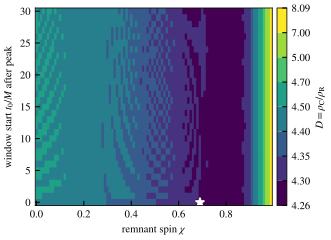
Figure 1 maps $D$ for the fundamental–overtone pair. Ignoring the correlations understates the required SNR by a factor of $4.25$ to $8.1$ over the entire physical range: there is no corner of spin or window choice where the shortcut is safe for this pair. At the GW150914-like point $(\chi ,t_0)=(0.69,0)$ the single-mode baseline declares the pair resolvable at $\rho \approx 71$, while the correlation-aware construction requires $\rho \approx 310$ (Table I). Both absolute thresholds grow steeply as the window start moves away from the peak and the overtone decays, but their ratio stays near $4.3$; the penalty is a property of the pair, not of the window. Across the sampled grid the frequency condition of Eq. 5 always sets the threshold (the damping-time condition never binds for either construction), so the thresholds reported here are frequency-resolution limited.

The structural driver is the overlap, and Eq. 8 shows what sets its size. At $\chi =0.69$ the closed form gives $\mu =0.8638$, matching the pipeline to four digits ($\kappa =13.7$); its equal-frequency limit is $0.8643$, so the $2.2\%$ frequency splitting shifts the overlap by well under $0.1\%$. So $\mu$, and with it the penalty, is set by the threefold damping-time difference almost alone, not by the frequency proximity the criterion is named for. At $\chi =0.99$, $\mu =0.878$ ($\kappa =15.4$). The analytic amplitude-only penalty of Eq. 7, ${(1-{\mu }^2)}^{-1/2}=1.98$, accounts for about half of the measured $D=4.29$; the rest comes from cross-parameter degeneracies that only the full $8\times 8$ analysis sees, and a per-parameter attribution of it has not been computed here. The $(2,2,0)$–$(3,3,0)$ control pair confirms pair-specificity: its splitting is large, $\mu$ is small, and the phase-median $D$ stays between $1.0$ and $2.0$ (median $1.4$; individual phases reach at most $2.1$), approaching unity at high spin (Fig. 2a).

Two consequences follow. First, the single-mode shortcut is tempting for the same reason the joint calculation is hard: the cross-terms [1]. Wherever it is used, it overstates the prospects of fundamental–overtone spectroscopy by a factor of about four in required SNR; forecasts built on the joint Fisher matrix, including the anchors here [1, 4, 5], are on the correct side of this gap. Second, both constructions place both-parameter resolvability of the $(2,2,0)\text{–}(2,2,1)$ pair at SNRs well beyond those of the events analyzed in the overtone dispute, consistent with that dispute remaining open [2, 3]; this work takes no position on that event.

VI Robustness

Figure 2: (a) $D$ at $t_0=0$ versus spin for the fundamental–overtone pair and the $(2,2,0)$–$(3,3,0)$ control. (b) Window-length dependence at $\chi =0.69$: shortening the window to $T=30M$ raises $D$ to about $6.4$; $T=100M$ differs from $T=60M$ by under $2\%$. Curves are medians over the 24-phase grid.

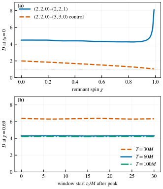
Three invariances are exact, not approximate. First, $D$ is independent of the amplitude ratio $R$: rescaling one mode’s amplitude rescales the corresponding rows and columns of both Fisher matrices, leaving every correlation coefficient unchanged, so the $1/\rho$-scaled $\sigma$’s shift identically in numerator and denominator of Eq. 6. The computed maps at $R=0.3$, $1$, and $3$ agree to better than ten significant digits everywhere on the grid. Second, the normalized template overlap $\mu$, and hence $\kappa$, is exactly invariant under window translation: shifting $t_0$ multiplies each template by a constant factor that cancels in the normalization. This is why Table I shows the same $\kappa$ at every $t_0$, and why the phase-median $D$ is nearly flat in $t_0$: its variation over the full window-start range is below $\pm 1\%$ at every spin. Third, with the white-noise product and windows scaled by $M$, the entire analysis is dimensionless and $D$ carries no mass dependence at all.

The relative phase is the one handle whose effect is not small pointwise, and it deserves stating as a limitation: individual-phase values of $D$ spread by about $22\%$ at the tabulated point and by up to $46\%$ at low spin about the reported medians. What is robust is the median itself: at the tabulated point the superseded four-sample grid (results v1) and the current 24-phase grid agree to five digits. Every threshold quoted here should therefore be read as a phase-median carrying a tens-of-percent phase spread, a property of the damped-sinusoid criterion itself rather than of this implementation. The window length behaves smoothly (Fig. 2): shortening to $T=30M$, which curtails the evolution that separates the two damping times, raises the penalty to $D\approx 6.4$, while lengthening to $T=100M$ shifts $D$ by under $2\%$. The one weighting not yet swept is a detector-shaped power spectral density, which breaks the mass invariance by introducing a physical frequency scale; whether $D$ itself moves qualitatively under a detector-shaped weighting is not answered here. That arm, and the anchor-exact horizon reproduction, are the declared next steps.

VII Conclusions

1. For the contested $(2,2,0)\text{–}(2,2,1)$ pair, ignoring the mode correlations in the Rayleigh resolvability criterion understates the required SNR by a factor of 4.25 to 8.1 (median over relative phase) across the entire astrophysical spin range and all analysis windows studied; at the GW150914-like point the thresholds are 71 versus 310. A well-separated control pair stays near or below a factor of 2.

2. The penalty is structural, not tuned: it is exactly independent of the mode amplitude ratio, exactly translation-invariant in its Gram diagnostic, and mass-invariant under white noise. Its scale is set by the template overlap, $\mu \approx 0.86$ to $0.88$, which the closed form of Eq. 8 ties to the damping-time ratio almost alone (the frequency splitting the criterion is named for contributes under one part in a thousand of the overlap), with cross-parameter degeneracies roughly doubling the analytic amplitude-only penalty of ${(1-{\mu }^2)}^{-1/2}\approx 2$. The medians are stable under phase-grid refinement, but individual-phase thresholds spread by tens of percent about them, and the white-noise inner product remains the analysis’s main untested assumption.

3. Practical recommendation: resolvability forecasts for overtone spectroscopy must draw their uncertainties from the joint Fisher matrix, as the anchor forecasts [1, 4, 5] do; assembling the same criterion from single-mode error formulas is unsafe for this pair by half an order of magnitude. The pipeline evaluates the correction in milliseconds per grid point; detector-PSD weighting and anchor-exact threshold reproduction are its next milestones.

References

- [1] E. Berti, V. Cardoso, and C. M. Will, “On gravitational-wave spectroscopy of massive black holes with the space interferometer LISA,” Phys. Rev. D, vol. 73, art. no. 064030, 2006, doi:10.1103/PhysRevD.73.064030. arXiv:gr-qc/0512160.
- [2] M. Isi, M. Giesler, W. M. Farr, M. A. Scheel, and S. A. Teukolsky, “Testing the no-hair theorem with GW150914,” Phys. Rev. Lett., vol. 123, art. no. 111102, 2019, doi:10.1103/PhysRevLett.123.111102. arXiv:1905.00869.
- [3] R. Cotesta, G. Carullo, E. Berti, and V. Cardoso, “Analysis of ringdown overtones in GW150914,” Phys. Rev. Lett., vol. 129, art. no. 111102, 2022, doi:10.1103/PhysRevLett.129.111102. arXiv:2201.00822.
- [4] I. Ota and C. Chirenti, “Black hole spectroscopy horizons for current and future gravitational wave detectors,” Phys. Rev. D, vol. 105, art. no. 044015, 2022, doi:10.1103/PhysRevD.105.044015. arXiv:2108.01774.
- [5] C. Shi, Q. Zhang, and J. Mei, “On the detectability and resolvability of quasi-normal modes with space-based gravitational wave detectors,” arXiv:2407.13110 [gr-qc], Jul. 2024.
- [6] E. Berti et al., “Black hole spectroscopy: from theory to experiment,” arXiv:2505.23895 [gr-qc], May 2025, submitted for publication.
- [7] J. L. Jaramillo, R. Panosso Macedo, and L. Al Sheikh, “Pseudospectrum and black hole quasi-normal mode (in)stability,” Phys. Rev. X, vol. 11, art. no. 031003, 2021, doi:10.1103/PhysRevX.11.031003. arXiv:2004.06434.
- [8] K. Destounis, R. Panosso Macedo, E. Berti, V. Cardoso, and J. L. Jaramillo, “Pseudospectrum of Reissner–Nordström black holes: Quasinormal mode instability and universality,” Phys. Rev. D, vol. 104, art. no. 084091, 2021, doi:10.1103/PhysRevD.104.084091. arXiv:2107.09673.
- [9] E. Gasperín and J. L. Jaramillo, “Energy scales and black hole pseudospectra: the structural role of the scalar product,” Class. Quantum Grav., vol. 39, no. 11, art. no. 115010, 2022, doi:10.1088/1361-6382/ac5054. arXiv:2107.12865.
- [10] L. C. Stein, “qnm: A Python package for calculating Kerr quasinormal modes, separation constants, and spherical-spheroidal mixing coefficients,” J. Open Source Softw., vol. 4, no. 42, art. no. 1683, 2019, doi:10.21105/joss.01683. arXiv:1908.10377.
papers/physics/urtc26/main.tex with LaTeXML
0.8.8. The typeset main.pdf is canonical. Every number
regenerates with scripts/compute_map.py.