Air Drag as a Metric Ruler: Physically Grounded
Monocular Speed Recovery and Its Observability Limits

Abstract

A single camera cannot tell a near, slow projectile from a far, fast one: depth is the axis it does not measure, while time is the axis it measures almost exactly. Quadratic air drag connects the two, since a projectile sheds a fraction $kv\mathrm{\Delta }t$ of its speed in every interval $\mathrm{\Delta }t$ with $k$ a known drag constant, so metric speed is effectively written into the timing of the slow-down. This principle was established in simulation for ballistic re-entry tracking; we realize it on commodity phone cameras, and report what we believe is the first ground-scale experimental metric validation of drag-based monocular speed estimation. We validate on 51 badminton shots spanning $59.1$–$311.0\mathrm{km}/\mathrm{h}$ ($v/v_{\mathrm{T}}$ $2.5$–$12.9$), scored against two separately built stereo rigs that share the estimator’s drag model form. We find that with a single launch-position constraint – an oracle pin taken from the stereo reference – the estimator reads 7.8% median absolute error, roughly flat across the speed range, while without any position input the free fit reads 18.3% and is biased high. The fragile element is the position–scale family (a farther, faster launch reproducing the same image track), not the drag cue, and a deployable net-plane constraint built from court geometry alone recovers 8.3% with no stereo input, close to the oracle, though like the oracle it reads one-sidedly high (median signed $+8.0\%$). Flat drives, already well conditioned, act as a built-in control: there the anchor changes almost nothing. The method’s scope comes down to one number, the fractional-decay integral $k{v}_{0}T\gtrsim 1$ (our validated events lie at $2.5$–$10.3$), with noise and frame count setting a higher practical threshold. Alongside our main results, we release the trajectories, video, calibrations and annotations as a benchmark.

1 Introduction

A calibrated camera fixes metric scale on its reference plane and nowhere else: above that plane, scaling position and velocity together leaves the image track unchanged, so one view cannot separate close-and-slow from far-and-fast. What, then, does a camera measure well? Time, almost perfectly – and quadratic air drag couples the two axes. In the drag-dominated regime a projectile loses a fraction $kv\mathrm{\Delta }t$ of its speed per interval $\mathrm{\Delta }t$, with $k=g/v_{\mathrm{T}}^2$ set by known aerodynamics, so the fractional decay rate is proportional to absolute speed: drag moves speed measurement onto the axis the camera measures best.

This observability principle is not ours to claim. Radar-based re-entry tracking established, by Fisher-matrix analysis entirely in simulation, that drag deceleration is what makes a ballistic target’s scale parameters estimable (Farina et al., 2002; Dodin et al., 2005, 2007); bearings-only target-motion analysis established separately that known or induced accelerations restore range to an angle-only track (Nardone and Aidala, 1981). In computer vision, known dynamics as a monocular metric reference has a gravity branch (Kim et al., 1998; Ribnick et al., 2009) and a drag branch, whose nearest member fits drag and Magnus terms to monocular table-tennis video, validated by reprojection without ground-truth speeds (Gossard et al., 2025). This paper supplies what the family lacks: the identifiability theory, and the first physical, angle-only test of the principle on commodity cameras at ground scale (Section 2).

Badminton is the test range, not the topic. The smash is the fastest racket-sport projectile relative to its terminal velocity, painted court lines supply a millimeter-specified calibration target, and shuttlecock dynamics collapse to a single parameter $v_{\mathrm{T}}$ (Chan and Rossmann, 2012; Cohen et al., 2014). The estimator consumes RGB video alone: a learned detector produces the pixel track, the physics fit turns it into metric speed, and a human corrects a few outlier frames; a two-phone stereo protocol, used only for evaluation, supplies the ground truth (Section 5).

Our contributions are as follows. (1) The first ground-scale experimental metric validation of drag-based monocular speed estimation on commodity cameras against a geometrically independent metric reference (Section 2): 51 shots over $59.1$–$311.0\mathrm{km}/\mathrm{h}$ ($v/v_{\mathrm{T}}$ $2.5$–$12.9$), ground-truthed by two independent stereo rigs under one pipeline and one readout-instant convention (Section 6.2). Anchored by a single launch-position constraint, an oracle pin from the stereo reference, the estimator holds 7.8% median absolute error, flat across the range. Without any position input the free fit reads 18.3% median; a deployable net-plane anchor, using court geometry alone, restores 8.3%, close to the oracle, though it shares the oracle’s one-sided over-read (Section 8). (2) A regime map for physics-as-scale: the gravity cue falls as $g/v^2$ while the drag cue grows as $kv$, unified on the $v/v_{\mathrm{T}}$ axis, with the necessary applicability criterion $k{v}_{0}T\gtrsim 1$ (Section 4), which also sorts other domains, from table tennis (borderline) to baseball (excluded). (3) A fragility and anchor analysis: backward extrapolation under quadratic drag makes the estimate hyper-sensitive to the contact instant, and the unanchored estimator shows the large one-sided errors this leverage predicts, while flat drives gain nothing from anchoring; the anchor removes the position family, not generic information (Sections 7 and 8). (4) A benchmark in preparation: 51 stereo-ground-truthed trajectories, released with video, calibrations, annotations, code and detector weights (Appendix G).

2 Related work

Gravity members.

Known physics can supply the metric constraint a single camera lacks, through gravity or through drag. Gravity is a known constant, so a monocular sequence that resolves curvature against it recovers scale: soccer-ball trajectories (Kim et al., 1998), the general projectile treatment (Ribnick et al., 2009), world-frame human motion (Shen et al., 2024), person height from video (Bieler et al., 2019). Gravity curvature is strongest at low speed over long flights; a fast, flat arc gives too little of it to read (Section 4).

Drag members.

That dissipative dynamics, not gravity, can carry scale comes from ballistic re-entry tracking, whose founding results are radar-based rather than passive. Farina et al. derive the Cramér–Rao bound for a radar tracking a re-entry ballistic target and compare nonlinear filters against it; their favored extended-Kalman-filter result assumes the ballistic coefficient known a priori rather than recovered from the measurements (Farina et al., 2002). Dodin et al. derive closed-form Fisher-information approximations for the same radar problem (range only, later range and bearing) and identify drag deceleration, not position, as what makes the ballistic coefficient itself estimable (Dodin et al., 2005, 2007), a simulation-only line taking part of its scale information from a modeled atmospheric density profile. The genuinely angle-only lineage is older, in bearings-only target-motion analysis: known or induced acceleration restores range observability to an otherwise unobservable angle-only track (Nardone and Aidala, 1981). Meteor astronomy applies the principle observationally, reading single-station speeds from atmospheric deceleration (Ceplecha et al., 1998), again hypersonic and against a modeled, altitude-varying atmosphere. At ground scale, sports computer vision uses drag inside the fitting model but takes scale from court or table geometry: MonoTrack fits a quadratic-drag flight model to monocular badminton video with endpoint pose priors (Liu and Wang, 2022); TT3D fits drag, Magnus lift and a bounce event to a monocular table-tennis trajectory by minimizing reprojection error (Gossard et al., 2025), extended in TT4D (Rahmanian et al., 2026); PMGS reconstructs projectile motion under a physics prior (Xu et al., 2025); and a deployed monocular badminton pipeline has separately been evaluated against a single fixed reference speed [anonymized system paper, withheld for double-blind review].

Our position.

TT3D is nearest in method: it too fits a drag-based ODE to a monocular ball track. But its scale comes from table geometry and the bounce event, and no recovered speed is checked against physical ground truth; the re-entry and meteor lines have the principle but no ground-scale validation. Isolating drag decay as the primary scale cue, deriving when it identifies speed (Section 4), and scoring recovered speeds against an independent stereo reference are, to our knowledge, new together.

3 Background

Dynamics.

A shuttlecock in flight feels gravity and quadratic drag, $m\dot{𝐯}=m𝐠-\frac{1}{2}\rho C_{D}A\parallel 𝐯\parallel 𝐯$. None of $\rho ,C_D,A,m$ need separate measurement: at terminal velocity the forces balance, $mg=\frac{1}{2}\rho C_{D}A{v}_{\mathrm{T}}^2$, so the model collapses onto a single measurable constant,

$$\dot{𝐯}=𝐠-\frac{g}{v_{\mathrm{T}}^2}\parallel 𝐯\parallel 𝐯.$$ (1)

We adopt $v_{\mathrm{T}}\approx 6.7\mathrm{m}/\mathrm{s}$ from the literature (Cohen et al., 2014; Chan and Rossmann, 2012) and use the same value in every fit (Section 6.2); the free-fall drops of Section 6.1 bracket it independently ($5.96$–$8.13\mathrm{m}/\mathrm{s}$ across release heights).

Observation model.

A camera with intrinsics and pose recovered from the court lines (a planar target with exactly known geometry) projects the trajectory $𝐩(t;𝜽)$, determined by the launch state $𝜽=({𝐩}_0,{𝐯}_0)\in {ℝ}^6$, through $\pi (\cdot )$ to image points. Detections $\{(t_i,{𝐱}_i)\}$ carry per-frame presentation timestamps (PTS), not a nominal $1/\mathrm{fps}$: consumer video is variable-frame-rate and the scale cue is read off the intervals between detections. The estimator integrates Eq. 1 with RK4 and solves for $𝜽$ by Levenberg–Marquardt under a Huber loss; contact speed is $s=\parallel 𝐯(t_c)\parallel$ at the contact instant $t_c$, with a 95% interval from the fit covariance propagated through the speed functional.

4 Why drag makes monocular speed identifiable

Every $(\alpha {𝐩}_0,\alpha {𝐯}_0)$ produces an identical image track under constant velocity, so what breaks the scaling family must be dynamics of known absolute magnitude. Gravity is the obvious candidate, deflecting an arc by $g{T}^2/2$ over a flight of duration $T$ – a weak cue for a short, nearly straight smash arc. Drag is far stronger. When ${(v/v_{\mathrm{T}})}^2\gg 1$ (about $108$ at $250\mathrm{km}/\mathrm{h}$), Eq. 1 reduces to $\dot{v}=-(g/v_{\mathrm{T}}^2)v^2$, and the per-frame fractional decay

$${\frac{\mathrm{\Delta }v}{v}|}_{\text{one frame}}\approx \frac{g}{v_{\mathrm{T}}^2}v\mathrm{\Delta }t$$ (2)

is proportional to $v$ itself: the faster the smash, the better conditioned the estimate.

Applicability criterion. The drag cue can supply metric scale only when the fractional-decay integral $k{v}_{0}T$ (the accumulated change in $1/v$ over the flight, scaled by $v_0$, with $k=g/v_{\mathrm{T}}^2$, $v_0$ the launch speed and $T$ the observed flight duration) is $\gtrsim 1$: the arc then sheds an order-one fraction of its launch speed (shed fraction $k{v}_{0}T/(1+k{v}_{0}T)$, i.e. half at $k{v}_{0}T=1$), rather than a small correction to it. The criterion is necessary, not sufficient: it says the cue is present, while click noise and frame count set the practical threshold. On this data the unanchored truncation ablation of Section 7 puts the empirical identifiability boundary at $\approx 250$–$400$ ms of arc ($k{v}_{0}T\approx 3$–$6$ at smash speeds), and $80$ ms prefixes with $k{v}_{0}T$ near $1$ scatter across an order of magnitude.

The criterion places the two physical cues on one footing. In short: normalized per unit time, gravity’s cue, of order $g/v$, weakens as speed grows while drag’s cue, the fractional decay rate $kv$ of Eq. 2, strengthens; they are equal exactly at $v=v_{\mathrm{T}}$ ($g/v=kv$ at $v^2=g/k$), so each regime is served by one cue: slow, curved flight by gravity, fast, flat flight by drag. All events validated here lie at $k{v}_{0}T$ of $2.5$–$10.3$: every observed arc sheds comfortably more than half its launch speed. The same arithmetic sorts other sports, from literature terminal velocities with typical launch speeds and flight times (Appendix C), against three bands fixed once here: $k{v}_{0}T\gtrsim 1$ viable (the necessary bar derived above), $0.3$–$1$ borderline (the cue is present but below this paper’s empirical threshold), excluded. A table-tennis smash gives $k{v}_{0}T\approx 0.7$–$1.5$, borderline to viable, pending validation at table-tennis noise and frame-count levels; a tennis serve before the bounce gives $0.4$–$0.7$, borderline; a baseball pitch gives $\approx 0.1$, excluded: a pitch sheds only a tenth of its speed, too little to carry scale.

A Fisher-information calculation (Appendix A) makes the comparison quantitative. It is an order-of-magnitude, aligned-case heuristic, with its two assumptions stated alongside the derivation, not an eigen-analysis of the full information matrix. Along the position–velocity scale ray gravity under-scales and drag over-scales the image track, and at equal geometry a gravity-only model’s speed variance exceeds the drag-aware one by ${(1+\mu c_d/c_g)}^2$, $\mu ={\parallel {𝐯}_0\parallel }^2/v_{\mathrm{T}}^2$ ($c_g,c_d$: image-plane visibilities of the two directions). At $250\mathrm{km}/\mathrm{h}$, $\mu \approx 108$ and an oblique view gives $\approx 1.2\times {10}^4$: a variance ratio, the square of the $\approx 100\times$ deceleration advantage.

The same mechanism exacts a price in time. Since $\dot{v}=-k{v}^2$ integrates to $1/v(t)=1/v_0+kt$, displacing the evaluation instant by $\delta$ rescales the answer by $1/(1+k{v}_0\delta )$, and backward extrapolation blows up in finite time: $v\to \mathrm{\infty }$ at $t=-1/(k{v}_0)$, only $65.9$ ms before contact at $250\mathrm{km}/\mathrm{h}$. One frame of contact-instant error at 30 fps moves a true $250\mathrm{km}/\mathrm{h}$ to $505.9$ or $166.0\mathrm{km}/\mathrm{h}$; at 240 fps the band is still $-6$ to $+7\%$, biased toward implausibly high readings, the worse direction for a deployed tool. The same bias appears empirically in Section 7.

5 The estimator

The full pipeline is automatic: a temporal detector fine-tuned on 22,000 hand-labeled frames (F1 $=0.86$, $1.61$ px median error, held-out clips) produces the track; a court-line engine recovers the camera; a breakpoint detector on log-image-speed splits at contact; the drag-aware fit of Section 3 produces speed with an interval. The split step’s accuracy is not separately evaluated (the real-data fits below split at the frame of peak annotated image speed, a proxy), and this compounds with the contact-instant leverage of Section 4: a one-frame split error at 240 fps rescales speed by $k{v}_0\mathrm{\Delta }t$ ($0.015$–$0.079$ across the pooled events), the same order as the anchored median of Section 7. A pooled refit with the split moved one frame later measures this: individual estimates move 7.9% median (max 19.4%), as the leverage predicts, while the mono-versus-reference comparison at the shifted instant differs by only 2.9% median. We find this more interesting than mere stability: the comparison is markedly better one frame later, suggesting the proxy sits about one frame early, making it the leading candidate for the anchored over-read (Section 7).

Simulation certifies what real events cannot: in a 252-cell sweep across viewpoint, frame rate, noise and speed, the estimator attains the Cramér–Rao bound in all 148 cells admitted by an a-priori conditioning rule ($\mathrm{RMSE}/\sqrt{\mathrm{CRLB}}\in [0.94,1.08]$, versus ratios up to $34$ in flagged cells, the scale-displaced failure Section 4 predicts), with interval coverage near nominal in both groups (Appendix B); simulation can only certify the estimator against its own generative assumptions. In the smash experiments below the per-frame positions are the detector’s own output with a small number of human-corrected outliers (the drops of Section 6.1 are tracked with no review), so reported speeds are those of the automatic pipeline up to that correction. A simplified variant ships in a consumer application, which is evidence of demand, not of accuracy.

6 Physical validation

6.1 Free-fall drops

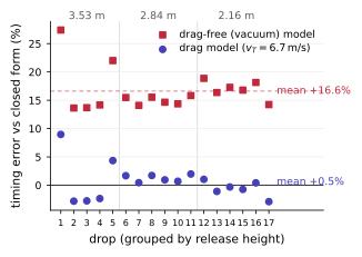
Synthetic experiments cannot validate the physical model, so we first test it with a tape measure: a shuttle released from rest obeys Eq. 1 with closed form $y(t)=(v_{\mathrm{T}}^2/g)\ln \cosh (gt/v_{\mathrm{T}})$. We dropped a feather shuttle from tape-measured heights of $2.16$, $2.84$ and $3.53$ m past surveyed wall markers, filmed at 120 fps with PTS timestamps and tracked automatically: $n=17$ usable drops, none excluded. The intervals between successive marker crossings match the closed form at the assumed $v_{\mathrm{T}}$ to $\mathbf{2.1}\%$ mean absolute error (max $9.0\%$, bias $+0.5\%$), while a drag-free model shows a systematic $+\mathbf{16.6}\%$ timing error on every single drop (Fig. 2, Appendix K): the drag term is load-bearing. Fitting each drop with $v_{\mathrm{T}}$ free recovers $v_{\mathrm{T}}=6.97\pm 1.13\mathrm{m}/\mathrm{s}$ (sample SD across drops; SEM $0.27\mathrm{m}/\mathrm{s}$), consistent with the assumed constant.

The per-height breakdown is exploratory (Appendix D): fitted $v_{\mathrm{T}}$ falls monotonically with release height, adjacent heights overlapping within about one sample SD. Since speed scales as $v_{\mathrm{T}}^2$, we record constant-$v_{\mathrm{T}}$ as a speed-dependent systematic of order $10\%$, outside any statistical interval; because the same fixed $v_{\mathrm{T}}$ enters both the stereo reference and the monocular estimator (Section 6.2), a speed-dependent refit would move both together and largely cancel in the reported error percentages while moving the absolute speeds. Two further caveats: a drop probes $v\lesssim v_{\mathrm{T}}$, and a drop from rest has no depth ambiguity, so this validates dynamics and timing, not monocular depth.

6.2 Two commodity stereo references across the speed regime

The speed reference is built entirely from consumer hardware, and built twice: two stereo rigs assembled independently in two capture sessions under one method and one fit pipeline. Each rig is two smartphones at 240 fps at crossing angles, clock-aligned by an audio clap and independently calibrated from human-labeled court-line junctions. Shuttle positions are annotated per frame in both views, and a single trajectory under Eq. 1, with $v_{\mathrm{T}}$ fixed at the literature value $6.70\mathrm{m}/\mathrm{s}$ used throughout the estimator, is fit jointly to all annotations of both cameras at their native timestamps; same-instant triangulation is unnecessary.

Session 1 (smash band). The close camera (iPhone 16 Pro, $720$p, $1.2$ px calibration rms) loses the shuttle $58$–$100$ ms after contact; the wide camera (iPhone 17 Pro, $1080$p, $4.7$ px) holds the longer view and carries the session-1 monocular fits. Both filmed in slow-motion mode corrected to $100\%$ playback, hence variable frame rate (Section 3). Three consistency checks support the reference; of course, none certifies its accuracy independently. First, the per-event clock offsets recovered by the joint fits agree across all events to within $0.7$ ms of a single value ($189.5$ ms); the audio clap gives $177.9$ ms, an $11.6$ ms discrepancy we attribute to a constant audio–video alignment offset, verified constant across events but not independently localized (Appendix E). Second, joint two-view fit residuals fall within $2.5$–$9.8$ px rms. Third, the reference does not presuppose the model it tests: a degree-4 polynomial with no drag term agrees with the physical fit to $1.6\%$ on the most densely annotated event. The session yields 10 events (nine smashes and one drop shot) spanning $69.1$–$311.0\mathrm{km}/\mathrm{h}$; seven of nine smash flights end at operator interference, so observed arcs are bounded by the capture protocol, not by play.

Session 2 (speed continuum). The second rig pairs camera 6461 (iPhone 17 Pro, wide) with camera 3236 (iPhone 16 Pro), whose view doubles as the monocular input, at a true $240$ fps. Clap offsets over the three simultaneous recordings close to within $\approx 1$ ms; court calibration gives $4$–$9$ px reprojection rms. The same player hit 66 events (drops, drives, half and full smashes), so the session covers $59.1$–$256.3\mathrm{km}/\mathrm{h}$ and, pooled with session 1, the full $59.1$–$311.0\mathrm{km}/\mathrm{h}$ range ($v/v_{\mathrm{T}}$ $2.5$–$12.9$, observed arcs $408.3$–$917.1$ ms). One corrected defect in the session-2 time base is disclosed in Appendix F; all session-2 fits and clap offsets use the corrected timestamps.

Which events count. An event enters the pooled statistics only if the joint stereo fit reproduces its own hand annotations in both views to better than 25 px rms: a gate on the reference, fixed before any monocular estimate was examined and not tuned to this dataset’s residual distribution (Appendix F). 25 of 76 annotated events fail it, 0 in session 1 and 25 in session 2 (Table 2, Appendix K): an annotation-quality difference between rigs, not a physics difference, and not a marginal call: any threshold between the worst accepted and best rejected per-view residual yields the identical pool (Appendix F). The surviving pool is 51 events (10 session 1, 41 session 2), and every statistic in Sections 7 and 8 is computed on it. In both sessions the monocular fits consume the same mono-view point track the reference is jointly fit to, so the gate screens the estimator’s input as well and the shared clicks correlate estimator and reference errors (unquantified); gating on the wide-view residual alone bounds that selection effect, and the pooled medians it yields are reported in Appendix F.

Speeds from two instruments are comparable only when read at the same instant: drag sheds $\approx 4\mathrm{km}/\mathrm{h}$ per millisecond at smash speed, so mixing readout conventions alone costs $\approx 3\%$. Every speed here, reference and estimator alike, is read at the first post-contact observation of the camera carrying the monocular fit; all speeds sit up to $\approx 17\mathrm{km}/\mathrm{h}$ below true racket-contact speed, which cancels in every comparison here but would matter for an absolute fastest-smash claim.

The reference’s uncertainty budget (term by term in Appendix E) spans systematics of $\approx \pm 3\%$ on the full arc to $\approx \pm 9\%$ on short arcs, a floor inherited by every error percentage quoted against it. We score below against a fixed $\pm 11\%$ band, a round number chosen ahead of scoring to sit modestly above the $\pm 9\%$ worst case, not derived from it; the within-band fractions are sensitive to that choice, so we read them as a coarse companion to the medians. One term sits outside the budget and must be carried explicitly: the constant-$v_{\mathrm{T}}$ model form (the order-$10\%$ speed-dependent systematic of Section 6.1) is shared between reference and estimator (both integrate Eq. 1 at the same fixed $v_{\mathrm{T}}$), so it cancels in every comparison, and the accuracy numbers of Sections 7 and 8 measure agreement with a drag-model reference, not distance from true speed. The model-free polynomial check constrains this on one event only, the only one annotated densely enough for a stable high-order fit, so errors against true speed could be larger by the order-$10\%$ shared term.

7 Against ground truth: accuracy, identifiability, honest intervals

We run the monocular estimator against the stereo reference on all 51 pooled events, every speed read at the common instant of Section 6.2. Figure 1 is the central result, signed speed error against $v/v_{\mathrm{T}}$; Table 1 pools the statistics and Table 3 lists every event (Appendix K). Throughout, “anchored” means oracle-anchored (Section 8), not a deployed reading.

Figure 1: Signed monocular speed error across the drag regime. Circles/upward triangles: unanchored; squares/downward triangles: oracle-anchored (Section 8); triangles are drives, hollow markers session-1 events; shaded band $\pm 11\%$, a fixed scoring band set modestly above the stereo-reference budget’s short-arc worst case (Section 6.2). Unanchored error is large and positive nearly everywhere; oracle-anchored error stays inside the band at every speed.

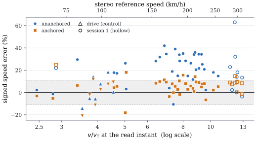
Oracle-anchored, the error is flat across the regime. With the launch position pinned (Section 8), the median absolute error is 7.8%, measured against a reference whose own systematic floor runs $\pm 3\%$ (full arc) to $\pm 9\%$ (short arcs; Section 6.2). 80.4% of events fall within $\pm 11\%$. By $v/v_{\mathrm{T}}$ quartile the median is 6.9 / 8.3 / 7.6 / 7.9% (Pearson $r=-0.20$ against $v/v_{\mathrm{T}}$): no trend, and the two rigs agree (8.8% session 1, 7.5% session 2). Once the position–scale family is removed, the residual error is small and flat across the regime. The anchored estimator is biased, not merely noisy: the median signed error is $+7.4\%$, an over-read on most events, and the worst event sits at 24.8% (event 12, the only session-1 drop shot; its $905$ ms arc rules out the short-arc degeneracy below; candidate mechanisms, unresolved, in Appendix J). The shared over-read is partially explained: the split-proxy refit of Section 5 points to a proxy sitting about one frame early as the leading candidate, with mono calibration scale and a residual depth family still open; we do not adjudicate here.

Anchored, drag still beats gravity-only, except in the top band. Rerunning the anchored harness with the drag term removed (gravity as the only dynamics) raises the pooled median absolute error from 7.8% to 12.4%, drag closer to the reference on 36 of 51 events. By $v/v_{\mathrm{T}}$ band: 6.4 versus 14.6% below $v/v_{\mathrm{T}}=5$ ($n=13$), 8.3 versus 14.6% from 5 to 8 ($n=13$), and parity at 7.9 versus 7.5% at $v/v_{\mathrm{T}}\ge 8$ ($n=25$). Drag is decisively better at low and mid $v/v_{\mathrm{T}}$; the top-band parity, reported as found, is consistent with the pinned read instant being nearly dynamics-free, drag’s demonstrated value there being to constrain the fit along the arc, not the instantaneous read (Appendix I).

Unanchored, the error is large and positively biased everywhere. The free fit’s median absolute error is 18.3% (only 25.5% within $\pm 11\%$; worst 62.9%), with median signed error $+18.3\%$: anchoring buys 2.35$\times$. These pooled numbers are confirmatory, on all 51 events; what follows is not. By quartile the error runs 10.9 / 26.2 / 28.2 / 14.8% (Pearson $r=0.19$); quartile composition is confounded with rig and shot label, so the shape is exploratory. Two statements are safe: this is not a test of the applicability criterion, since every pooled event has $k{v}_{0}T\ge 2.5$ and what fails is the conditioning of the position–scale family, not the cue; and the one-sided sign follows from the asymmetric backward extrapolation of Section 4. The magnitude is consistent with, but not derived from, the same contact-instant leverage: one frame of readout error rescales a reading by $\approx k{v}_0\mathrm{\Delta }t$ (Section 5), so 18.3% is equivalent to several frames of effective launch mislocation.

Drives are the built-in control. On flat, well-conditioned drive geometry (n=7), anchoring slightly degrades accuracy: 7.7% unanchored versus 9.3% anchored, a 0.83$\times$ “gain”: the free fit needs no help there, so the pin can only add the reference’s own launch-position error. Where the family is poorly conditioned the anchor pays instead: drops 2.93$\times$ (n=8), smashes 2.55$\times$ (n=24), half smashes 4.64$\times$ (n=12), on small per-category counts carrying no confidence adjectives (Appendix J).

The rest of the state comes free. Direction needs none of this machinery: the anchored launch direction errs 0.43^∘ in elevation and 0.40^∘ in azimuth (medians), the anchored landing point 0.20 m median from the stereo fit’s over 51 events; this is cross-instrument consistency, not ground truth (Appendix J). Speed is the one quantity that needed the drag cue.

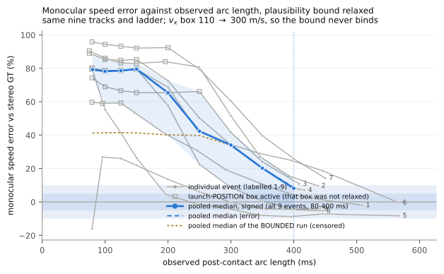
Identifiability, by ablation. Refitting each session-1 event unanchored on progressively shorter prefixes of its own track (Fig. 4) isolates observed arc length with everything else fixed. Pooled absolute error first falls inside $\pm 10\%$ near $400$ ms of arc and never reaches $\pm 5\%$; per-event spread at fixed arc is large ($3$–$43\%$ at $300$ ms), so arc length predicts the population, not an individual measurement. Below $\approx 250$ ms the metric scale is unidentifiable: with bounds relaxed, the nine $80$ ms session-1 fits scatter across an order of magnitude in speed, and these absurd optima fit the pixels better than plausible-speed fits ($3.5$ vs $8.1$ px rms), the flat likelihood direction of Section 4: goodness of fit is actively misleading near the degeneracy. Under the deployed $110\mathrm{m}/\mathrm{s}$ plausibility bound the same fits saturate there: a guardrail converting divergence into saturation, not an estimator property.

The confidence interval under-covers, for a structural reason. Propagating the fit covariance through the speed functional for the nine session-1 smash fits gives narrow intervals ($\pm 6$ to $\pm 42\mathrm{km}/\mathrm{h}$) that cover the reference on only 5 of 9 events, with misses of $2$–$8.4\sigma$: the covariance propagates click noise only, while calibration scale, the drag constant, the readout instant and click-to-click correlation sit outside it (Appendix B). The consequence for deployment is a-priori refusal on insufficient arc rather than a wider error bar (a gate the simulation rule of Section 5 implements, unevaluated per event here).

8 Repairing the degeneracy: the launch-position anchor

The failure mode is a one-parameter family: a faster launch slightly farther from the camera reproduces the same pixels, so one world-space constraint should collapse it. The repair is the launch-position anchor, the launch pinned to the stereo trajectory’s position at the common instant: an oracle that measures the ceiling of what any independent launch fix could buy, not a deployed reading. That ceiling is the cross-regime curve of Section 7: 7.8% median absolute error, 80.4% within $\pm 11\%$, flat in $v/v_{\mathrm{T}}$ (Table 1). One circularity must be stated: the pin comes from the same joint stereo fit, at the same read instant, as the ground-truth speed, so anchored error partly measures that fit’s self-consistency. A jack-knife bounds it: re-deriving each pin from stereo fits on the odd and even frame half-splits moves the anchored speed 0.2% median (1.1% worst): the circularity is negligible.

The pin must be tight: $\pm 0.30$ m of slack costs a third of the median gain and most of the within-band gain (median 11.4% versus 7.8%; 47.1% within $\pm 11\%$ versus 80.4%, signed $+10.8\%$), so any deployment substitute for the oracle must localize the contact point to decimeters, not to a meter.

How close can a deployable anchor come to the oracle? Below it sits a ladder of candidates (harness and per-event detail in Appendix H). Pose-based pins are limited by cohort priors, not by detection: a stance pin fails at $+44.7\%$ mean because contact sits $\approx 0.8$ m of reach from the feet, and closing that reach with a published segment chain recovers $+13.1\%$ (session-1 smashes, $n=9$).

The strongest candidate needs no pose detection: the fit is parametrised by its crossing of the official net plane, with $x=6.70$ m enforced exactly at a fitted crossing instant (crossing position on the plane, velocity and crossing time free), using only the monocular track and court geometry. Under the unified pipeline, over all 51 gate-passing events of both sessions (all 51 cross the plane inside the observed span), it reads 8.3% median absolute error pooled (6.1% over the 10 session-1 events, 9.0% over the 41 session-2 events, 71% inside $\pm 11\%$), against 7.8% for the oracle pin on the same events: with no stereo input, the deployable anchor lands close to the oracle pooled, halving the free fit’s 18.3%, though the oracle keeps a wider within-band margin (80.4% versus 71%). Note that the crossing-state parametrisation has the same six free parameters as the free fit; the constraint’s information enters through requiring a crossing inside the observed span, together with the dynamics, not through dimensional reduction. The residual error is one-sided (median signed $+8.0\%$), and its worst event, at $+26.4\%$, is the session-1 drop that is also the oracle pin’s worst event, which supports a shared systematic there. But the session split is not so clean: session-1 net-plane bias is $+1.1\%$ against the oracle’s session-1 bias, while session 2 runs $+8.9\%$ against a smaller oracle bias, so session 2 carries an excess that could equally be a net-plane or calibration defect. We have not resolved which. And unlike the pinned read instant of Section 7, drag is load-bearing here: rerunning the net-plane harness with the drag term removed collapses the median to 33.8% (signed $-33.8\%$), drag closer to the reference on 48 of 51 events – the plane fixes where the arc crosses, but only the decay says how fast. Plane-constrained fits stay pixel-clean right or wrong, so a deployment must gate on the criterion and observed arc, not on fit residual (Appendix H). The decomposition also matters beyond this testbed, where launch position is often a surveyed constant, not a moving contact (Section 9).

Finally, viewing direction: a virtual-camera sweep (Appendix H) yields $1$–$3\%$ mean error at every azimuth when the full arc is in frame at 240 fps; angle dependence re-emerges only as samples thin.

9 Conclusion

Re-entry tracking showed in simulation that dissipative dynamics carry a ballistic target’s scale; bearings-only analysis, that known accelerations restore range to an angle-only track. We give the combined principle its first physical, angle-only test on a phone, where quadratic drag writes true speed into the timing of a decelerating arc. Anchoring the launch state on the scaling family it belongs to (the oracle pin of Section 8) holds the monocular speed error at a median 7.8%, flat in speed, across $59.1$–$311.0\mathrm{km}/\mathrm{h}$ on two independent stereo rigs and 51 ground-truthed flights, and we find that a deployable net-plane anchor built from court geometry alone lands close to that ceiling (8.3%, Section 8). The drag term separates from a gravity-only fit at low and mid $v/v_{\mathrm{T}}$, reaching top-band parity where the pinned read instant is nearly dynamics-free (Section 7). What we export is not a badminton speed but the necessary criterion $k{v}_{0}T\gtrsim 1$: the arc must shed an order-one fraction of its own speed, with noise and frame count setting a higher practical threshold (Section 4). More than any single number, we hope to convey that a camera’s clock is a metric instrument.

Limitations.

All ground-truth events come from one player and one venue, and shuttle type is fixed within a session. The stereo reference is self-consistent but not cross-validated by an instrument outside its own pipeline. Two dependencies from Section 6.2 bound the reported errors: the reference shares the estimator’s drag model and fixed $v_{\mathrm{T}}$, so those errors measure agreement with that model family, not distance from true speed; and the monocular fits consume the same mono-view annotations the reference is fit to, so estimator and reference errors are not fully independent. The anchored $+7.4\%$ one-sided bias is a partially explained shared systematic (the split proxy sitting about one frame early is the leading candidate, Sections 5 and 7); the net-plane anchor shares it (median signed $+8.0\%$), its recommended deployment gate is not evaluated per event here, and the anchored drag-free ablation reaches top-band parity (Section 7). Fit-quality screening rejects 25 of 66 session-2 and 0 of 10 session-1 events before any speed is reported (Section 6.2): the validated set is a filtered subset of what was filmed. The tracks are detector output with human outlier correction; uncorrected tracks were not retained, so the correction’s residual effect is unquantified. Reported intervals treat calibration, $v_{\mathrm{T}}$ and the time base as exact and are structurally too narrow (Section 7); the azimuth sweep is simulation only, no conditioning gate runs on the real events, and rolling shutter is uncorrected.

Broader impact and ethics.

What we validate is a coupling, not a sport statistic: dissipative dynamics of known constant convert the axis a camera measures well (time) into the one it does not (metric scale), and each way of turning that coupling around is its own problem. Run forward it yields speed and, via depth along the ray, passive range; the criterion is checkable in advance. Volcanology already deploys three synchronized high-speed cameras because one view cannot resolve motion along its axis (Taddeucci et al., 2012; Gaudin et al., 2016); there the launch is a surveyed vent, so the anchored 7.8% applies with no oracle (we have not computed $k{v}_{0}T$ for a Strombolian bomb). Inverted, the same observability makes the drag constant the estimand (single-view discrimination by ballistic coefficient) or the time base itself: $g$ and $k$ enter at different powers of time, so a decelerating track over-determines its own clock – a playback-rate check for video forensics. This is the ballistic member of a family that treats cameras as time-axis instruments, with the recovery of sound from micron vibrations (Davis et al., 2014); none of these inversions is evaluated here. Spin is out of scope (a shuttlecock is spin-stabilized); TT3D’s Magnus term (Gossard et al., 2025) under the same Fisher treatment is next. The misuse risk, over-trust in a too-short arc, is answered by a-priori refusal (Section 7); the input is video of objects, not people.

Appendix A Fisher-information derivation for the scale ray

Fisher information makes the gravity–drag comparison of Section 4 quantitative to order of magnitude, and it matters what the information is about: the unknown is the full launch state $𝜽$, not speed alone. The variance-ratio result below is an order-of-magnitude, aligned-case heuristic, not a bound derived from an eigen-analysis of the full information matrix; it rests on two unstated-strength assumptions, made explicit here: (i) the scale ray dominates the projected speed variance, so other directions in $𝜽$ contribute negligibly to $\mathrm{Var}(\widehat{s})$; and (ii) the gravity and drag image-motion signals are treated as additive in magnitude, which holds in the aligned case where both act along comparable image directions and can fail by sign cancellation otherwise. Under Gaussian pixel noise $\sigma$, $ℐ(𝜽)={\sigma }^{-2}{\sum }_i{𝐉}_i^{\top }{𝐉}_i$ with ${𝐉}_i=\partial \pi (𝐩(t_i;𝜽))/\partial 𝜽$, and the delta method projects onto the speed functional, $\mathrm{Var}(\widehat{s})\ge \nabla s^{\top }{ℐ}^{-1}\nabla s$. The derivation is short. Along the scale ray $\alpha \mapsto (\alpha {𝐩}_0,\alpha {𝐯}_0)$ the pinhole map (camera at the origin) satisfies $\pi (\alpha 𝐱)=\pi (𝐱)$, and to second order in $t$ the scaled trajectory is $\alpha [{𝐩}_0+{𝐯}_{0}t+\frac{1}{2}(𝐠/\alpha +\alpha {𝐚}_d)t^2]$ with drag acceleration ${𝐚}_d=-(g/v_{\mathrm{T}}^2)\parallel {𝐯}_0\parallel {𝐯}_0$ of magnitude $\mu g$, $\mu ={\parallel {𝐯}_0\parallel }^2/v_{\mathrm{T}}^2$: position and velocity scale exactly, gravity under-scales, drag over-scales. Differentiating at $\alpha =1$, the image motion per unit scale is $\frac{1}{2}{t}^2\mathrm{\Pi }({𝐚}_d-𝐠)$ ($\mathrm{\Pi }$ the projection Jacobian), of magnitude proportional to $g(c_g+\mu c_d)$ for image-plane visibilities $c_g,c_d\in [0,1]$ of the gravity and velocity directions (the norm of each unit direction’s projection onto the image plane; amplitudes treated as additive, the aligned case). Scale information is this signal squared and a gravity-only model keeps only $g{c}_g$, so if the scale ray dominates the projected speed variance, gravity-only speed variance exceeds drag-aware variance at equal geometry by ${(1+\mu c_d/c_g)}^2$. At $250\mathrm{km}/\mathrm{h}$, $\mu \approx 108$; substituting $c_d/c_g\approx 1$ (an oblique view with both directions comparably visible) gives ${(1+108)}^2\approx 1.2\times {10}^4$, not a best case: the ratio is unbounded as $c_g\to 0$ and falls to parity as $c_d\to 0$. This is a variance ratio, the square of the $\approx 100\times$ deceleration advantage.

Appendix B Simulation envelope of the estimator

The 252-cell sweep of Section 5 crosses viewpoint, frame rate, noise and speed, with 500 Monte-Carlo trials per cell ($\approx 3\%$ Monte-Carlo error per ratio). A cell is admitted iff its predicted relative bound $\sqrt{\mathrm{CRLB}}/s\le 5\%$, computable from geometry, frame rate, noise and nominal speed before any data are seen; 148 cells are admitted, 104 flagged. In admitted cells $\mathrm{RMSE}/\sqrt{\mathrm{CRLB}}\in [0.94,1.08]$; in flagged cells the ratio reaches $34$. Intervals cover at $94.5\%$ in admitted cells and $93.6\%$ in flagged ones ($94.1\%$ pooled, $95\%$ nominal): $\mathrm{RMSE}/\sqrt{\mathrm{CRLB}}$ compares the error to the bound, coverage compares the interval to the error.

On the real events the picture differs (Section 7): the real-data misses of $2$–$8.4\sigma$ are unrelated to arc length and not one-sided, and inflating every real-event interval $\approx 4\times$ would cover all nine session-1 smashes. A local covariance models the noise you assumed, not the errors that dominate: simulation draws its noise from the assumed model, so coverage holds there while calibration scale, the drag constant, the readout instant and click-to-click correlation (all outside the covariance) break it on real data.

Appendix C Other-sports arithmetic for the applicability criterion

The cross-domain values quoted in Section 4 use literature terminal velocities (Cohen et al., 2014) with typical launch speeds and observable flight times: a table-tennis smash ($v_{\mathrm{T}}\approx 9$–$10\mathrm{m}/\mathrm{s}$, $v_0\approx 25$–$30\mathrm{m}/\mathrm{s}$, $T\approx 0.3$–$0.4$ s) gives $k{v}_{0}T\approx 0.7$–$1.5$; a tennis serve before the bounce ($v_{\mathrm{T}}\approx 21\mathrm{m}/\mathrm{s}$, $v_0\approx 50$–$60\mathrm{m}/\mathrm{s}$, $T\approx 0.4$–$0.5$ s) gives $0.4$–$0.7$; a baseball pitch ($v_{\mathrm{T}}\approx 35$–$40\mathrm{m}/\mathrm{s}$, $v_0\approx 40\mathrm{m}/\mathrm{s}$, $T\approx 0.4$ s) gives $\approx 0.1$. These are necessary-side screenings only: whether a domain that passes the bare $\gtrsim 1$ bar is identifiable in practice depends on its click noise and frame count, which on our data pushed the empirical threshold to $k{v}_{0}T\approx 3$–$6$ (Section 7).

Appendix D Per-height drop analysis

The per-height breakdown of Section 6.1 is exploratory and, on its own evidence, still open: fitted $v_{\mathrm{T}}$ falls monotonically with release height ($8.13\pm 0.79$, $6.65\pm 0.36$, $5.96\pm 0.83\mathrm{m}/\mathrm{s}$ from $2.16$, $2.84$, $3.53$ m; mean $\pm$ sample SD, $n=6$, $6$, $5$), with adjacent heights overlapping within about one sample SD and no trend test reported: faster flight suggests a smaller $v_{\mathrm{T}}$, more drag than any constant reproduces. The direction is opposite to feather-skirt compression, which would push fitted $v_{\mathrm{T}}$ up (Cohen et al., 2014; Chan and Rossmann, 2012); we flag the trend as suggestive rather than established. A speed-dependent refit would move reference and estimator together (Section 6.2) and largely cancel in the reported error percentages; it would move the absolute reference and estimated speeds themselves by the differential sensitivity of Appendix E, not the pooled anchored median.

Appendix E Stereo-reference uncertainty budget

The three terms of Section 6.2: the formal per-event $\pm 1$–$2\mathrm{km}/\mathrm{h}$ is statistical only ($\lesssim 0.7\%$); calibration scale contributes $\approx \pm 2$–$3\%$; and the fixed $v_{\mathrm{T}}$ enters through a measured sensitivity: refits at the per-height extremes of Section 6.1 move the stereo speeds by $-10$ to $-30$ percent per $\mathrm{m}/\mathrm{s}$, through which the drop SEM ($0.27\mathrm{m}/\mathrm{s}$) propagates as $\approx \pm 3$ to $\pm 8\%$. We use the SEM of the pooled $v_{\mathrm{T}}$ fit, not the larger per-drop sample SD ($1.13\mathrm{m}/\mathrm{s}$) or the per-height spread ($5.96$–$8.13\mathrm{m}/\mathrm{s}$, Appendix D), because this term is meant to capture how precisely we know the single constant $v_{\mathrm{T}}$ actually used in every fit, reference and estimator alike; the speed-dependent trend across heights is a separate, shared systematic already carried outside this budget (Section 6.1), not sampling uncertainty on the constant. In quadrature the systematics span $\approx \pm 3\%$ on the full arc to $\approx \pm 9\%$ on short arcs.

Clock offset.

The $11.6$ ms gap between the session-1 clap offset ($177.9$ ms) and the value the joint fits recover ($189.5$ ms) was not independently localized, for example by re-clapping at a second position, which would separate a fixed processing delay from an acoustic-path term of a few meters. What we did verify is that the offset is constant across events, to within $0.7$ ms, which is the property the fit needs: a per-event-varying offset would appear as scatter in the recovered offsets, and it does not.

Appendix F Reference gate, time base, disposition and selection effect

Session-2 time base.

One corrected defect is disclosed: the original frame extraction computed each trimmed clip’s frame times from the trim boundary rather than the container’s presentation timestamps, giving every trim its own constant inter-view offset. Frame times were re-extracted, and all session-2 fits, including the clap offsets quoted in Section 6.2, use the corrected time base.

Threshold and disposition.

The 25 px gate of Section 6.2 is a round number consistent with prior annotation-noise experience on this pipeline, not tuned to this dataset’s residual distribution. It is not marginal: the worst accepted per-view residual is 14.7 px (median 7.0) and the best rejected is 28.6 px, so any threshold between them yields the identical pool and the specific value 25 is not load-bearing. Of the 25 rejections, 10 events fail on the wide view alone, 8 on both views, and 7 on the mono view alone (Table 2).

Because the mono view is both a gated view and the estimator’s input, the gate screens the estimator’s input as well as the reference. Gating on the wide-view residual alone re-admits the 7 mono-view failures ($n=58$) and moves the pooled medians from 18.3% to $19.9\%$ unanchored and 7.8% to $8.3\%$ anchored, an upper bound on the degradation, since the re-admitted references are themselves fit to the failed annotations.

Appendix G Released artifacts

Code, calibration data, drop-test videos, annotations, per-event fits, and the ablation and anchor-variant artifacts (priors, audit logs, refits) will be released on publication, together with the fine-tuned detector weights and the 22,000-frame detector training annotations (Section 5). The human-corrected point tracks used in the smash experiments will be released; the pre-correction tracks were not retained for this data (a limitation noted in Section 9), and we commit to retaining and releasing both raw and corrected tracks for future capture sessions.

Appendix H Anchor variants and viewpoint sweep

Stance pin.

On the session-1 events, pinning the launch at the smasher’s annotated feet (court-plane homography, an independent $2.43$ m contact-height prior (Phomsoupha and Laffaye, 2015), no stereo input) errs $\approx +45\%$, worse than not anchoring, because contact sits a consistent reach vector from the feet ($+0.72\pm 0.20$ m netward, $-0.36\pm 0.11$ m across, measured against the stereo launch points as a diagnostic only), and $15$ px of stance error already moves the answer by tens of km/h. Recovering the launch point from stance therefore needs a cohort reach model rather than better foot detection; we release the measurements and do not pursue the route.

Reach chain.

Closing the feet-to-contact reach with published segment ratios (Winter, 2009), the legal racket maxima (BWF, 2025), the measured stature and the same height prior (every constant fixed before any fit) predicts a $0.63$ m horizontal reach against the observed $0.81\pm 0.19$ m, and scores $+13.1\%$ mean over the nine session-1 events ($+8.3\%$ over the eight longest arcs, parity with the oracle pin’s $+7.8\%$ mean and $8.2\%$ mean absolute error on the same eight). The chain under-predicts the reach; cohort priors, not foot detection, are what limit a stance-based anchor. These stance, reach and contact-ray diagnostics are computed under the earlier session-1 convention noted in Section 8, not the unified pipeline, and are quoted for the pose ladder only.

Contact-ray pin.

A stance-free contact-ray pin (the contact pixel’s camera ray intersected with the height prior) removes the reach problem but inherits the prior: $+12.4\%$ mean, every event high. Self-diagnosis differs by mechanism: pin-anchor fit residuals track their own error (correlation $0.97$ for the stance pin), while plane-constrained fits stay pixel-clean right or wrong ($-0.22$) and must be gated on plane-miss distance instead ($+0.60$).

Viewpoint.

Placing virtual cameras around the session-1 ground-truth trajectories (full arc in frame, 240 fps, $3$ px noise, $11$ m distance) and sweeping azimuth from directly behind ($0^{\circ }$) to side-on (${90}^{\circ }$) yields mean errors of $1$–$3\%$ at every angle. With the full arc at high frame rate, viewpoint is nearly irrelevant; the Fisher angle-dependence re-emerges exactly where samples become scarce (at 30 fps the same sweep gives $16\%$ directly behind vs. $7\%$ side-on, and short arcs fail at any angle). The guidance: stand far enough back, at any convenient angle, that the entire flight stays in frame, which a rear-diagonal phone placement achieves naturally, as our cameras did.

Appendix I Why the drag-free baseline reaches parity in the top band

The band-by-band gravity-only comparison of Section 7 shows drag ahead at low and mid $v/v_{\mathrm{T}}$ and at parity for $v/v_{\mathrm{T}}\ge 8$. We report that parity as found and offer one interpretation, labeled as such: with the launch position pinned, the speed read at the common instant is nearly dynamics-free (approximately depth times angular rate), so the drag model’s contribution is to constrain the fit along the arc rather than at the read instant, and on the fastest, flattest arcs the two dynamics constrain it about equally well. The lower bands, where the unpinned parts of the trajectory matter more, are where the drag term pays.

Appendix J Direction and landing point

Against the stereo fit, the anchored launch direction errs 0.43^∘ median in elevation and 0.40^∘ in azimuth (worst 2.11^∘ and 3.13^∘); even unanchored, 1.30^∘ and 1.56^∘. The fitted model also yields a full trajectory and a landing point: over all 51 events the anchored landing point sits 0.20 m median from the stereo fit’s (worst 0.76 m), with flight time to landing off by 4.8 ms median. Two caveats: where the observed arc ends before the floor (most events), both landing points are model extrapolations, so this is cross-instrument consistency, not ground truth; and everything beyond the launch state is carried by the drag ODE, whose form is constrained only by the drop test of Section 6.1.

Per-category anchor gains.

The drive control of Section 7 should not be read as an accuracy ranking: both drive numbers (7.7% unanchored, 9.3% anchored) are middling relative to the other categories’ anchored errors, and the claim is only that anchoring leaves drives roughly where it found them. The anchor removes the position–scale family specifically; the per-category counts behind the reported gains are small.

Event 12.

The worst anchored event (24.8%; the only session-1 drop shot) has a $905$ ms arc, ruling out the short-arc degeneracy of Section 7. The likelier contributors are its annotation density (session-1 drops were not annotated as densely as the smashes that dominate the session) and the low-speed $v_{\mathrm{T}}$ mismatch flagged in Section 6.1; this event’s $v/v_{\mathrm{T}}=2.9$ is the lowest in session 1, closest to where fitted $v_{\mathrm{T}}$ departs furthest from the fixed constant; we do not resolve which dominates.

Appendix K Per-event tables and supplementary figures

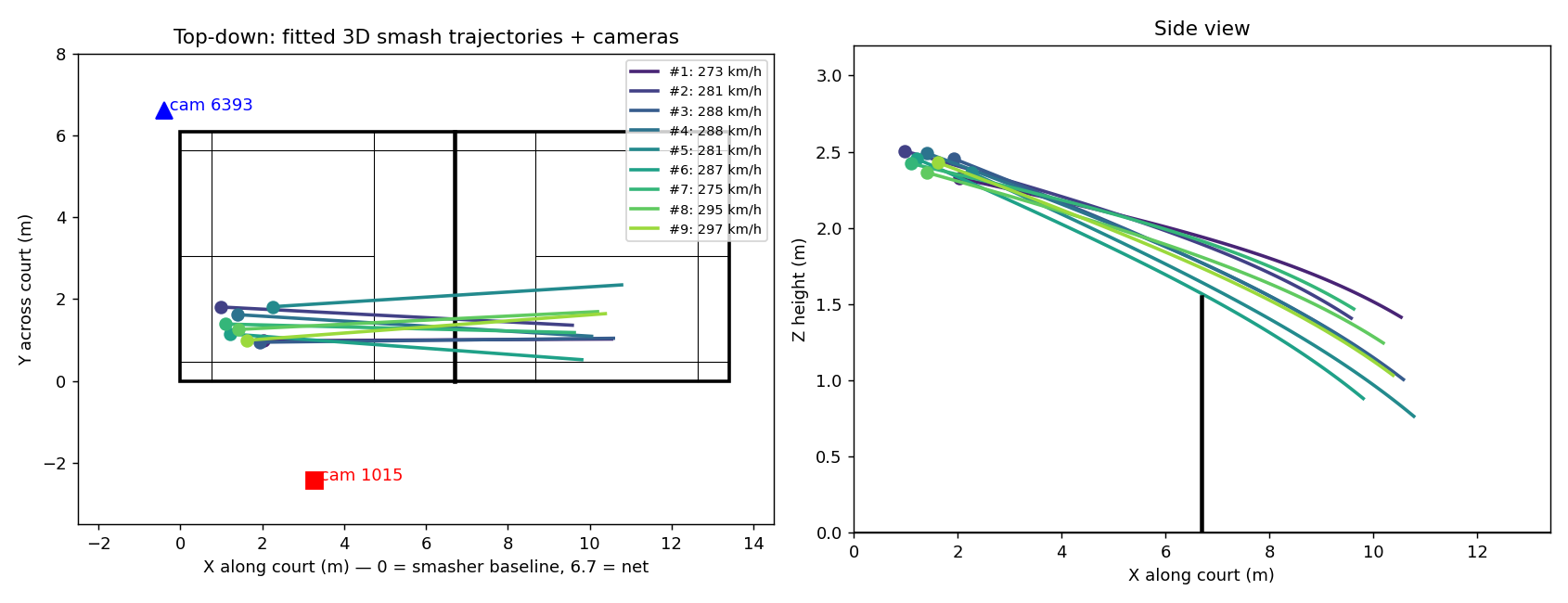
Table 1 is the pooled accuracy table for Section 7, including the within-band fractions by shot label, by $v/v_{\mathrm{T}}$ quartile and by rig. Table 2 lists every rejected event with per-view residuals and failure cause; Table 3 lists every event that passes the gate, with reference, unanchored, anchored and slack-anchored speeds. Figure 2 shows the free-fall validation of Section 6.1; Fig. 3 shows the session-1 stereo geometry of Section 6.2; Fig. 4 is the truncation ablation discussed in Section 7.

Table 1: Pooled monocular accuracy against the stereo reference. Median absolute speed error and the fraction of events inside $\pm 11\%$ (the widest stereo-reference budget of Section 6.2), over all 51 events that pass the stereo-residual gate. “Unanchored” is the free monocular fit; “anchored” pins the launch position to the stereo trajectory at the common instant; “slack” relaxes that pin to $\pm 0.30$ m. Bands are quartiles of $v/v_{\mathrm{T}}$.

		median $|$error$|$ (%)		within $\pm 11\%$ (%)
Subset	$n$	unanch.	anchored	unanch.	anchored
All	51	18.3	7.8	25.5	80.4
by shot label
drive	7	7.7	9.3	57.1	57.1
drop	8	17.5	6.0	37.5	62.5
half	12	28.3	6.1	25.0	83.3
smash	24	20.6	8.1	12.5	91.7
by $v/v_{\mathrm{T}}$ quartile
$2.5$–$4.6$	12	10.9	6.9	50.0	66.7
$4.7$–$7.8$	13	26.2	8.3	23.1	76.9
$7.8$–$9.3$	13	28.2	7.6	0.0	84.6
$9.5$–$12.9$	13	14.8	7.9	30.8	92.3
by rig
session 1	10	16.0	8.8	30.0	80.0
session 2	41	18.8	7.5	24.4	80.5

Table 2: Disposition of every rejected event. An event enters the pooled statistics only if the joint stereo fit reproduces the hand annotations in both views to better than 25 px rms; the gate is applied to the reference, before any monocular estimate is examined. 25 of 76 annotated events fail it, all in session 2. The stereo speed of a rejected event is not a usable reference and is shown only to identify the failure.

Event	Shot	rms wide (px)	rms mono (px)	(stereo km/h)	Cause
3	drive	41	6	98	wide-view annotation
6	drive	8	49	195	mono-view annotation
15	drop	74	17	94	wide-view annotation
16	drop	16	31	147	mono-view annotation
19	drop	16	76	579	mono-view annotation
20	drop	18	82	187	mono-view annotation
21	drop	152	24	53	wide-view annotation
25	drop	19	44	132	mono-view annotation
27	drop	10	60	129	mono-view annotation
29	drop	74	8	88	wide-view annotation
32	drop	80	13	86	wide-view annotation
42	half	18	82	240	mono-view annotation
44	half	53	61	376	both views
46	half	29	17	230	wide-view annotation
53	half	54	43	290	both views
54	half	41	28	249	both views
55	half	53	95	581	both views
59	smash	64	9	133	wide-view annotation
62	smash	88	15	158	wide-view annotation
63	smash	743	212	15	both views
65	smash	47	26	557	both views
66	smash	73	17	186	wide-view annotation
68	smash	162	29	132	both views
77	smash	73	10	79	wide-view annotation
89	smash	49	115	584	both views

Table 3: Every event that passes the stereo-residual gate, sorted by reference speed. Speeds in km/h, read at the mono camera’s first post-contact observation. $T$ is the observed arc; $k{v}_{0}T$ is the fractional speed shed over it. Session-1 events are marked $†$. Text statistics use unrounded fits.

Event	Shot	$T$ (ms)	$v/v_{\mathrm{T}}$	$k{v}_{0}T$	Stereo GT	Unanch.	Anchored	Slack
31	drop	900	2.5	3.2	59	60	57	59
23	drop	796	2.8	3.3	67	66	64	66
12†	drop	905	2.9	3.8	69	84	86	84
30	drop	917	3.4	4.6	82	106	87	91
1	drive	479	3.5	2.5	85	73	68	70
13	drive	530	3.8	2.9	91	86	89	86
5	drive	521	3.9	3.0	93	107	104	107
2	drive	600	3.9	3.5	95	90	84	87
9	drive	580	4.1	3.5	99	107	102	106
8	drive	508	4.4	3.2	105	125	113	117
7	drive	446	4.6	3.0	110	110	120	115
18	drop	613	4.6	4.1	110	130	115	120
17	drop	613	4.7	4.2	113	133	119	125
28	drop	721	5.0	5.3	121	153	99	104
14	drop	558	5.1	4.1	122	126	144	137
35	half	521	6.4	4.9	155	199	168	176
91	smash	684	6.6	6.6	160	211	176	184
36	half	546	6.9	5.5	166	236	185	194
37	half	538	7.0	5.5	169	227	184	192
47	half	555	7.2	5.8	173	179	166	173
64	smash	742	7.3	8.0	177	210	191	199
41	half	438	7.4	4.7	179	160	178	171
39	half	546	7.5	6.0	181	252	191	202
57	half	559	7.7	6.3	185	213	190	200
74	smash	525	7.8	6.0	187	251	207	219
43	half	438	7.8	5.0	188	241	184	192
49	half	525	8.0	6.2	193	261	223	237
52	half	463	8.2	5.5	197	253	213	224
67	smash	613	8.3	7.5	201	230	206	218
69	smash	621	8.5	7.7	206	259	217	227
87	smash	488	8.7	6.2	209	233	217	227
45	half	421	8.7	5.4	211	283	213	223
85	smash	592	8.8	7.6	213	289	243	258
90	smash	667	8.9	8.7	214	258	235	247
78	smash	438	9.1	5.8	219	294	239	250
83	smash	512	9.1	6.8	220	267	239	252
71	smash	467	9.3	6.4	224	301	235	246
84	smash	434	9.3	5.9	225	282	243	255
75	smash	684	9.5	9.5	229	277	247	262
58	half	625	9.6	8.8	232	237	217	226
73	smash	521	10.2	7.8	247	291	252	265
92	smash	471	10.6	7.3	256	294	270	284
7†	smash	450	11.7	7.7	282	347	307	325
5†	smash	567	11.9	9.9	287	293	308	293
3†	smash	408	12.2	7.3	293	478	336	354
2†	smash	438	12.2	7.8	294	389	320	340
1†	smash	509	12.3	9.2	297	297	300	297
4†	smash	417	12.3	7.5	298	339	325	339
6†	smash	567	12.4	10.3	299	354	329	347
11†	smash	442	12.9	8.3	311	300	307	300
10†	smash	446	12.9	8.4	311	353	337	353

Figure 2: Free-fall validation. Per-drop timing error against the closed-form drag solution, all $n=17$ drops by release height; the drag model (blue) sits at $+0.5\%$ mean error, the vacuum model (red) is biased $+16.6\%$ and misses on every drop.

Figure 3: Session-1 stereo reference. Top-down and side views of the fitted 3D trajectories with the two camera positions (legend device ids: 1015 close, 6393 wide); all launch $2.2$–$2.5$ m high and cross the net at $1.6$–$1.9$ m.

Figure 4: Truncation ablation, uncensored. Each session-1 event refit on progressively longer prefixes of its own track; grey curves are per-event error, the accent curve the pooled median, bands $\pm 5$ and $\pm 10\%$; the faint reference is the pooled median under the deployed $110\mathrm{m}/\mathrm{s}$ bound, whose short-arc plateau is the bound itself. Pooled error crosses $\pm 10\%$ near $400$ ms; below $\approx 250$ ms scale is unidentifiable and short-arc fits diverge while fitting the pixels better than plausible speeds.

References

- Kim et al. (1998) T. Kim, Y. Seo, and K.-S. Hong. Physics-based 3D position analysis of a soccer ball from monocular image sequences. Proc. ICCV, pages 721–726, 1998.
- Ribnick et al. (2009) E. Ribnick, S. Atev, and N. Papanikolopoulos. Estimating 3D positions and velocities of projectiles from monocular views. IEEE TPAMI, 31(5), 2009.
- Cohen et al. (2014) C. Cohen, B. Darbois-Texier, G. Dupeux, E. Brunel, D. Quéré, and C. Clanet. The aerodynamic wall. Proc. R. Soc. A, 470, 2014.
- Chan and Rossmann (2012) C. M. Chan and J. S. Rossmann. Badminton shuttlecock aerodynamics: synthesizing experiment and theory. Sports Engineering, 15(2):61–71, 2012.
- Phomsoupha and Laffaye (2015) M. Phomsoupha and G. Laffaye. The science of badminton: Game characteristics, anthropometry, physiology, visual fitness and biomechanics. Sports Medicine, 45(4):473–495, 2015.
- Winter (2009) D. A. Winter. Biomechanics and Motor Control of Human Movement. Wiley, 2009.
- BWF (2025) Badminton World Federation. Laws of Badminton, Law 4 (BWF Statutes, Section 4.1), version 5.0, in force 26 April 2025.
- Gossard et al. (2025) T. Gossard, A. Ziegler, and A. Zell. TT3D: Table tennis 3D reconstruction. CVSports Workshop, CVPR, 2025.
- Liu and Wang (2022) P. Liu and J.-H. Wang. MonoTrack: Shuttle trajectory reconstruction from monocular badminton video. CVSports Workshop, CVPR, 2022.
- Dodin et al. (2005) P. Dodin, P. Minvielle, and J.-P. Le Cadre. Re-entry vehicle tracking observability and theoretical bound. Proc. 8th Int. Conf. on Information Fusion (FUSION), pages 197–204, 2005.
- Dodin et al. (2007) P. Dodin, P. Minvielle, and J.-P. Le Cadre. Estimating the ballistic coefficient of a re-entry vehicle. IET Radar, Sonar & Navigation, 1(3):173–183, 2007.
- Nardone and Aidala (1981) S. C. Nardone and V. J. Aidala. Observability criteria for bearings-only target motion analysis. IEEE Transactions on Aerospace and Electronic Systems, AES-17(2):162–166, 1981.
- Farina et al. (2002) A. Farina, B. Ristic, and D. Benvenuti. Tracking a ballistic target: comparison of several nonlinear filters. IEEE Transactions on Aerospace and Electronic Systems, 38(3):854–867, 2002.
- Ceplecha et al. (1998) Z. Ceplecha, J. Borovička, W. G. Elford, D. O. ReVelle, R. L. Hawkes, V. Porubčan, and M. Šimek. Meteor phenomena and bodies. Space Science Reviews, 84(3–4):327–471, 1998.
- Shen et al. (2024) Z. Shen, H. Pi, Y. Xia, Z. Cen, S. Peng, Z. Hu, H. Bao, R. Hu, and X. Zhou. World-grounded human motion recovery via gravity-view coordinates. SIGGRAPH Asia (Conference Track), 2024.
- Bieler et al. (2019) D. Bieler, S. Günel, P. Fua, and H. Rhodin. Gravity as a reference for estimating a person’s height from video. ICCV, 2019.
- Xu et al. (2025) Y. Xu, J. Zhang, Y. Chen, D. Wang, L. Yu, and C. He. PMGS: Reconstruction of projectile motion across large spatiotemporal spans via 3D Gaussian splatting. arXiv:2508.02660, 2025.
- Rahmanian et al. (2026) N. Rahmanian, D. Kienzle, T. Gossard, D. Kalaria, R. Lienhart, and S. Sastry. TT4D: A pipeline and dataset for table tennis 4D reconstruction from monocular videos. arXiv:2605.01234, 2026.
- Taddeucci et al. (2012) J. Taddeucci, P. Scarlato, A. Capponi, E. Del Bello, C. Cimarelli, D. M. Palladino, and U. Kueppers. High-speed imaging of Strombolian explosions: The ejection velocity of pyroclasts. Geophysical Research Letters, 39:L02301, 2012.
- Taddeucci et al. (2017) J. Taddeucci, M. A. Alatorre-Ibargüengoitia, O. Cruz-Vázquez, E. Del Bello, P. Scarlato, and T. Ricci. In-flight dynamics of volcanic ballistic projectiles. Reviews of Geophysics, 55(3):675–718, 2017.
- Davis et al. (2014) A. Davis, M. Rubinstein, N. Wadhwa, G. J. Mysore, F. Durand, and W. T. Freeman. The visual microphone: passive recovery of sound from video. ACM Transactions on Graphics, 33(4):79:1–79:10, 2014.
- Gaudin et al. (2016) D. Gaudin, J. Taddeucci, B. F. Houghton, T. R. Orr, D. Andronico, E. Del Bello, U. Kueppers, T. Ricci, and P. Scarlato. 3-D high-speed imaging of volcanic bomb trajectory in basaltic explosive eruptions. Geochemistry, Geophysics, Geosystems, 17(10):4268–4275, 2016.