Does the air resistance on a falling badminton shuttlecock increase with the square of its speed?

1 Research design

1.1 Research question

A shuttlecock dropped from a first-floor window drifts down at walking pace rather than accelerating all the way: for a body this light with a skirt this open, drag is not a correction to $F_g=mg$ but a term of comparable size. The data booklet gives only Stokes’ law, $F_d=6\pi \eta rv$, for a small sphere creeping through a viscous fluid — the opposite regime.

How does the square of the speed, $v^2$, of a feather badminton shuttlecock released from rest depend on the vertical displacement $s$ through which it has fallen, over the range $s=0$ to $2.4\mathrm{m}$ in still indoor air?

The independent variable is $s$, the dependent variable $v^2$; both are read off the same video of the same fall, so each pair comes from one measurement rather than two separately timed ones. A drag force proportional to $v^2$ and a drag-free fall predict measurably different shapes for that relationship, so measuring it decides between them. Deriving the quadratic prediction below produces one unknown constant, the terminal velocity $v_{\mathrm{T}}$, which the same measurement returns.

1.2 Background physics

Step 1: why the drag force goes as ${𝒗}^{\mathrm{𝟐}}$.

Falling at speed $v$ with frontal area $A$ through air of density $\rho$, the shuttle sweeps out in time $\mathrm{\Delta }t$ a cylinder of air of volume

$$V=Av\mathrm{\Delta }t.$$ (1)

By $\rho =m/V$ that cylinder has mass

$$m_{\text{air}}=\rho V=\rho Av\mathrm{\Delta }t,$$ (2)

and the shuttle shoves it aside, giving it a speed of order $v$. By $p=mv$ the momentum handed over is

$$\mathrm{\Delta }p=m_{\text{air}}v=\left(\rho Av\mathrm{\Delta }t\right)v=\rho A{v}^2\mathrm{\Delta }t,$$ (3)

so by $F=\mathrm{\Delta }p/\mathrm{\Delta }t$ the air pushes back with

$$F_d=\frac{\mathrm{\Delta }p}{\mathrm{\Delta }t}=\frac{\rho A{v}^2\mathrm{\Delta }t}{\mathrm{\Delta }t}=\rho A{v}^2.$$ (4)

This fixes the form but not the factor, since the air is not all given precisely the speed $v$; that factor is absorbed into a dimensionless drag coefficient, conventionally written with a $\frac{1}{2}$:

$$F_d=\frac{1}{2}\rho C_{D}A{v}^2.$$ (5)

For a feather shuttle $C_D\approx 0.6$ [3]: doubling the speed quadruples the drag.

Step 2: Newton’s second law.

Downwards positive, the net force is $F_{\text{net}}=mg-\frac{1}{2}\rho C_{D}A{v}^2$, so by $F=ma$

$$ma=mg-\frac{1}{2}\rho C_{D}A{v}^2,$$ (6)

and dividing every term by $m$,

$$a=g-\frac{\rho C_{D}A}{2m}{v}^2.$$ (7)

The acceleration depends on the speed already reached, so it is not constant — which is why the suvat equations cannot be applied to the fall as a whole.

Step 3: four unknowns into one.

As the shuttle speeds up the drag term grows until it balances the weight; then $a=0$ and the speed stops changing at the terminal velocity $v_{\mathrm{T}}$. Setting $a=0$, $v=v_{\mathrm{T}}$ in Equation 6,

$$0=mg-\frac{1}{2}\rho C_{D}A{v}_{\mathrm{T}}^2,mg=\frac{1}{2}\rho C_{D}A{v}_{\mathrm{T}}^2,$$ (8)

$$v_{\mathrm{T}}^2=\frac{2mg}{\rho C_{D}A},v_{\mathrm{T}}=\sqrt{\frac{2mg}{\rho C_{D}A}}.$$ (9)

Dividing Equation 8 by $m$ isolates the awkward group in Equation 7,

$$g=\frac{\rho C_{D}A}{2m}{v}_{\mathrm{T}}^2⟹\frac{\rho C_{D}A}{2m}=\frac{g}{v_{\mathrm{T}}^2},$$ (10)

and substituting it back,

$$a=g-\frac{g}{v_{\mathrm{T}}^2}{v}^2⟹\boxed{a=g(1-\frac{v^2}{v_{\mathrm{T}}^2}).}$$ (11)

One unknown remains, $v_{\mathrm{T}}$, so the model makes a testable prediction once that constant is fixed. At release $v=0$ so $a=g$ (ordinary free fall); as $v\to v_{\mathrm{T}}$ the bracket vanishes so $a\to 0$.

Step 4: predicting ${𝒗}^{\mathrm{𝟐}}$ against $𝒔$.

Since $a$ changes as the shuttle falls, $v^2=u^2+2as$ cannot be applied across the whole drop — but it can across a step short enough that $v$, and so $a$, barely changes. Cutting the fall into steps of $\mathrm{\Delta }s$ and labelling them $i=0,1,2,\mathrm{\dots }$ with $v_0=0$ at $s=0$, the acceleration across step $i$ is

$$a_i=g\left(1-\frac{v_i^2}{v_{\mathrm{T}}^2}\right),$$ (12)

and $v^2=u^2+2as$ with $u=v_i$, $a=a_i$, $s=\mathrm{\Delta }s$ gives

$$\boxed{v_{i+1}^2=v_i^2+2a_i\mathrm{\Delta }s.}$$ (13)

Applying the two in turn builds $v^2$ at every displacement, for any trial $v_{\mathrm{T}}$. The first two steps at $\mathrm{\Delta }s=0.10\mathrm{m}$ and $v_{\mathrm{T}}=6.5\mathrm{m}{\mathrm{s}}^{-1}$ (so $v_{\mathrm{T}}^2=42.25{\mathrm{m}}^2{\mathrm{s}}^{-2}$):

$v_0^2$ $=0$ released from rest

$a_0$ $=9.81\left(1-\frac{0}{42.25}\right)=9.81\mathrm{m}{\mathrm{s}}^{-2}$

$v_1^2$ $=0+2(9.81)(0.10)=1.96{\mathrm{m}}^2{\mathrm{s}}^{-2}$ at $0.10\mathrm{m}$

$a_1$ $=9.81\left(1-\frac{1.96}{42.25}\right)=9.36\mathrm{m}{\mathrm{s}}^{-2}$

$v_2^2$ $=1.96+2(9.36)(0.10)=3.83{\mathrm{m}}^2{\mathrm{s}}^{-2}$ at $0.20\mathrm{m}$

Free fall over the same $0.20\mathrm{m}$ gives $2gs=3.92{\mathrm{m}}^2{\mathrm{s}}^{-2}$: a $2\%$ gap this early, widening with every step. The analysis uses $\mathrm{\Delta }s=1\mathrm{mm}$; halving it moves $v^2$ at the end of the longest fall by $0.013\%$, far below the measurement uncertainty, so the calculation is converged.

Step 5: imperfect releases do not matter.

Equation 13 gives one curve of $v^2$ against $s$ per $v_{\mathrm{T}}$: the speed depends only on how far the shuttle has fallen, not on when it was let go. A shuttle leaving the hand with a small downward speed $u$ is therefore not on a different curve but further along the same one, at the point where it reaches $u$. Shifting the measured displacements by a constant $s_0$ — where the model reaches $u$ — makes them coincide exactly. This is the advantage of $(s,v^2)$ over $(t,s)$, where a mistimed release biases every later measurement.

1.3 Hypothesis

The graph of $v^2$ against $s$ should leave the origin along $v^2=2gs$, gradient $2g=19.62\mathrm{m}{\mathrm{s}}^{-2}$, then bend below that line and flatten towards $v_{\mathrm{T}}^2$. Taking the published feather-shuttle value $v_{\mathrm{T}}\approx 6.7\mathrm{m}{\mathrm{s}}^{-1}$ [2, 3], the plateau is expected near $45{\mathrm{m}}^2{\mathrm{s}}^{-2}$, and stepping Equation 13 to $s=2.4\mathrm{m}$ predicts $v^2\approx 30{\mathrm{m}}^2{\mathrm{s}}^{-2}$ against the $2gs=47{\mathrm{m}}^2{\mathrm{s}}^{-2}$ of constant acceleration. The two differ by over a third, far beyond any plausible measurement error.

1.4 Variables

Table 1: Variables and how each was fixed or measured.

Independent	Displacement $s$, $0\mathrm{m}$ to $2.4\mathrm{m}$, sampled at $120\mathrm{Hz}$ rather than at a few discrete settings; obtained from wall markers surveyed with a tape measure.
Dependent	$v^2$, from the gradient of the displacement–time graph over a short window of frames, then squared.
Controlled	Shuttle: one feather shuttle [TO CONFIRM: brand, grade, mass on a balance] throughout, so $C_{D}A/m$ in Equation 9 is fixed.
	Air: indoors [TO CONFIRM: room; doors, windows and fans shut?], fixing $\rho$ and excluding draughts.
	Orientation: [TO CONFIRM: how held; allowed to settle cork-down?] — falling skirt-first would present a different $A$.
	Camera: tripod-mounted, not moved within a clip, framing and $120\mathrm{fps}$ unchanged, so one calibration serves every drop in it.
	Release: dropped, never thrown, level with the chosen marker.

1.5 Apparatus and method

Feather shuttlecock [TO CONFIRM: brand, mass]; four strips of pink tape as wall markers; tape measure [TO CONFIRM: type, smallest division]; smartphone camera [TO CONFIRM: model] on a tripod, portrait video 3840 pixels tall at $120\mathrm{fps}$ with per-frame timestamps.

1. Tape the four markers to the wall in a vertical line at $139\mathrm{in}$, $112\mathrm{in}$, $85\mathrm{in}$ and $39.37\mathrm{in}$ above the floor ($3.531\mathrm{m}$, $2.845\mathrm{m}$, $2.159\mathrm{m}$, $1.000\mathrm{m}$), the tape measure [TO CONFIRM: run and read how?] at each mark. These four heights are the only route from pixels to metres.

2. Set the tripod [TO CONFIRM: distance] back, square to the wall, markers running down the long axis of the frame. Two framings were used: one for the $2.16\mathrm{m}$ drops, one shared by the $2.84\mathrm{m}$ and $3.53\mathrm{m}$ drops. All four markers are visible in both.

3. Hold the shuttle with its cork level with the chosen marker [TO CONFIRM: how steadied?] and release by opening the fingers, not pushing.

4. Record one continuous clip per release height, so every drop in it shares a calibration and an unbroken timestamp sequence. Repeat several times at each of $2.16\mathrm{m}$, $2.84\mathrm{m}$ and $3.53\mathrm{m}$, giving three fall distances over which to test the same model.

5. Track each clip frame by frame: locate the shuttle as the moving object in the marked strip and record its centroid in pixels with that frame’s own timestamp, read from the file rather than assumed to be $1/120$ s apart — phone video is variable-frame-rate and occasionally drops a frame.

6. Exclusions, fixed in advance: keep a track only if it stays inside the calibrated strip for at least 25 frames, and discard the first three frames of each release, where the hand is still in frame and pulls the centroid off the shuttle. Seventeen drops met these conditions and all seventeen are reported.

Safety, ethical and environmental.

The $3.53\mathrm{m}$ marker is above head height, so [TO CONFIRM: how reached, what precaution]. The shuttle is too light to injure and the fall zone was kept clear. A person visible in the raw footage between drops is removed by the background-median step and appears in no analysed frame; no personal data is recorded. The tape was removed afterwards and the shuttle returned to use.

2 Data analysis

2.1 From pixels to metres

The wall recedes towards the top of the frame, so equal heights subtend fewer pixels the higher they are; ignoring this would put a systematic distortion into $s$. For a camera looking along a straight line the exact relation between height $H$ and pixel row $y$ is

$$H=\frac{\alpha y+\beta }{\gamma y+1}.$$ (14)

Multiplying by $(\gamma y+1)$ gives $H\gamma y+H=\alpha y+\beta$, so $\alpha y+\beta -H\gamma y=H$, which is linear in $\alpha$, $\beta$, $\gamma$. Four markers of known height give four such equations for three unknowns, solved by least squares. Being over-determined, the leftover residuals test the model: the worst across both framings is $1.7\mathrm{cm}$, about $0.5\%$ of the shortest fall.

2.2 Raw data

Table 2: Time $t$ to fall a displacement $s$ from release, as the mean over the drops at each release height $\pm$ the standard deviation across those repeats. A dash means the shuttle did not fall that far in that framing. $\mathrm{\Delta }s=\pm \mathrm{\hspace{0.17em}0.02}\mathrm{m}$, $\mathrm{\Delta }t=\pm \mathrm{\hspace{0.17em}0.004}\mathrm{s}$ (Table 3).

Displacement $s$ / m	Time since release $t$ / s
	from $2.16\mathrm{m}$	from $2.84\mathrm{m}$	from $3.53\mathrm{m}$
0.25	0.220 $\pm$ 0.005	0.231 $\pm$ 0.072	0.181 $\pm$ 0.028
0.50	0.310 $\pm$ 0.005	0.331 $\pm$ 0.071	0.285 $\pm$ 0.037
0.75	0.384 $\pm$ 0.004	0.405 $\pm$ 0.071	0.368 $\pm$ 0.042
1.00	0.451 $\pm$ 0.007	0.471 $\pm$ 0.071	0.431 $\pm$ 0.041
1.25	—	0.532 $\pm$ 0.071	0.496 $\pm$ 0.042
1.50	—	0.588 $\pm$ 0.073	0.554 $\pm$ 0.044
1.75	—	0.641 $\pm$ 0.072	0.612 $\pm$ 0.044
2.00	—	—	0.662 $\pm$ 0.045
2.25	—	—	0.713 $\pm$ 0.047

Reading down any column of Table 2, equal increments of displacement take steadily less time — as they must, since the shuttle is speeding up — but the decrease slows markedly, the first sign that the acceleration is not constant.

2.3 Processing

Speed is the gradient of the displacement–time graph, taken at frame $i$ across a window of 9 frames centred on it:

$$v_i=\frac{s_{i+4}-s_{i-4}}{t_{i+4}-t_{i-4}}.$$ (15)

The window matters: a gradient between neighbouring frames would divide $2\mathrm{cm}$ of position uncertainty by the $8.3\mathrm{ms}$ between them and return metres per second of scatter, whereas over 9 frames the baseline is eight times longer and the scatter eight times smaller, while $0.067\mathrm{s}$ is still short enough that the speed changes little across it. Each drop is then fitted with Equation 13 for two quantities: $v_{\mathrm{T}}$, and the offset $s_0$ of Section 1.

2.4 Uncertainties

Table 3: Uncertainties and where they come from.

$\mathrm{\Delta }H=\pm \mathrm{\hspace{0.17em}0.5}\mathrm{in}$ $=\pm \mathrm{\hspace{0.17em}1.3}\mathrm{cm}$	By judgement: the tape’s reading error plus the difficulty of holding it vertical over $3.5\mathrm{m}$. On the $139\mathrm{in}$ baseline that is a $0.36\%$ scale error; since $v_{\mathrm{T}}\propto \sqrt{\text{length}}$, the exponentiation rule with $n=\frac{1}{2}$ halves it to $0.18\%$ on $v_{\mathrm{T}}$.
$\mathrm{\Delta }s=\pm \mathrm{\hspace{0.17em}0.02}\mathrm{m}$	Not pixel noise but the shuttle being an extended object whose centroid is not its centre of mass and whose outline changes as it rotates. $2\mathrm{cm}$ is roughly the shuttle’s own length, a conservative bound; the $1.7\mathrm{cm}$ calibration residual sits inside it.
$\mathrm{\Delta }t=\pm \mathrm{\hspace{0.17em}0.004}\mathrm{s}$	Half a frame interval at $120\mathrm{fps}$. Each frame carries its own timestamp, so this is a quantisation bound, not a reaction time — no human starts or stops a clock anywhere here. Over a $0.7\mathrm{s}$ fall, $0.6\%$.
$\mathrm{\Delta }v$, $\mathrm{\Delta }\left(v^2\right)$	Propagated through Equation 15: a quotient of two differences, so absolute uncertainties add in numerator and denominator, then fractional uncertainties add for the quotient, then double for the square. Worked below.
$\mathrm{\Delta }{v}_{\mathrm{T}}$	From the spread of the 17 drops, not from propagation: the drop-to-drop scatter is several times what propagating $\mathrm{\Delta }s$ and $\mathrm{\Delta }t$ predicts, so the propagated figure would overstate the precision. The sample standard deviation is used rather than the standard error of the mean, because the scatter reflects real physical variation between drops (Section 4).

2.5 Sample calculation

Worked in full for the drop from $3.53\mathrm{m}$ at the frame where $s=1.00\mathrm{m}$; scripts/analyse.py repeats it for all 1124 points.

1. Pixel row to height.

At $y=1635.3$, Equation 14 gives $H=100.59\mathrm{in}=100.59\times 0.0254=2.555\mathrm{m}$. The shuttle was first tracked at $H_0=140.00\mathrm{in}=3.556\mathrm{m}$, so

$$s=H_0-H=3.556-2.555=1.001\mathrm{m}.$$

2. Speed.

The frames four either side are $(t,s)=(0.3917\mathrm{s},0.8676\mathrm{m})$ and $(0.4583\mathrm{s},1.1336\mathrm{m})$, so by Equation 15

$$v=\frac{1.1336-0.8676}{0.4583-0.3917}=\frac{0.2660}{0.0666}=3.99\mathrm{m}{\mathrm{s}}^{-1},v^2=15.9{\mathrm{m}}^2{\mathrm{s}}^{-2}.$$

3. Its uncertainty.

Both differences are subtractions, so absolute uncertainties add:

$$\mathrm{\Delta }(s_{i+4}-s_{i-4})=0.02+0.02=0.04\mathrm{m},$$

$$\mathrm{\Delta }(t_{i+4}-t_{i-4})=0.004+0.004=0.008\mathrm{s}.$$

For the quotient, fractional uncertainties add:

$$\frac{\mathrm{\Delta }v}{v}=\frac{0.04}{0.2660}+\frac{0.008}{0.0666}=0.150+0.120=0.270,\mathrm{\Delta }v=1.1\mathrm{m}{\mathrm{s}}^{-1}.$$

Squaring uses $\mathrm{\Delta }y/y=|n\mathrm{\Delta }a/a|$ with $n=2$:

$$\frac{\mathrm{\Delta }(v^2)}{v^2}=2(0.270)=0.540,\mathrm{\Delta }(v^2)=8.6{\mathrm{m}}^2{\mathrm{s}}^{-2}.$$

This is a worst case: it assumes the $2\mathrm{cm}$ sits at one end of the window and the opposite error at the other, whereas that bound is dominated by the shuttle’s changing outline, which varies frame to frame and so largely cancels across the window. The observed scatter is nearer $1{\mathrm{m}}^2{\mathrm{s}}^{-2}$, so Figure 1 plots the standard error within each bin and $8.6{\mathrm{m}}^2{\mathrm{s}}^{-2}$ is kept only as the guaranteed limit on one point.

4. The two models there.

Constant acceleration gives $v^2=2gs=2(9.81)(1.001)=19.6{\mathrm{m}}^2{\mathrm{s}}^{-2}$; stepping Equation 13 to $s=1.001\mathrm{m}$ at $v_{\mathrm{T}}=6.45\mathrm{m}{\mathrm{s}}^{-1}$ gives $15.7{\mathrm{m}}^2{\mathrm{s}}^{-2}$. The measured $15.9{\mathrm{m}}^2{\mathrm{s}}^{-2}$ lies $0.2{\mathrm{m}}^2{\mathrm{s}}^{-2}$ from the drag prediction and $3.7{\mathrm{m}}^2{\mathrm{s}}^{-2}$ below free fall.

2.6 Graphical analysis

Figure 1: $v^2$ against $s$, pooled over all 17 drops and binned in $0.1\mathrm{m}$ intervals; error bars are the standard error within each bin. Dashed: constant acceleration, $v^2=2gs$. Solid: Equation 13 stepped at $v_{\mathrm{T}}=6.45\mathrm{m}{\mathrm{s}}^{-1}$. Lower panel: the residual from each model, same scale.

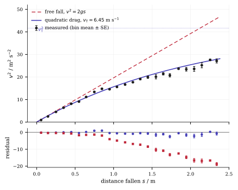
Near release the two models agree, and so does the data.

A straight line through the points with , where drag has barely acted, has gradient $(18.1\pm 0.5)\mathrm{m}{\mathrm{s}}^{-2}$ against the $2g=19.62\mathrm{m}{\mathrm{s}}^{-2}$ that constant acceleration requires, and intercept $-0.097{\mathrm{m}}^2{\mathrm{s}}^{-2}$, consistent with zero as a release from rest demands. The apparatus reproduces ordinary kinematics where ordinary kinematics applies.

It reads low by exactly the amount drag predicts.

That gradient is $3.3$ standard uncertainties below $2g$, which alone would look like a discrepancy. Stepping Equation 13 at $v_{\mathrm{T}}=6.45\mathrm{m}{\mathrm{s}}^{-1}$ over the same range and fitting a straight line to that asks what the drag model itself would return: $18.22\mathrm{m}{\mathrm{s}}^{-2}$, within $0.2\sigma$ of the measurement. Drag has already removed a few percent of $v^2$ by $0.30\mathrm{m}$ and the measurement sees precisely that much.

Over the whole fall, free fall fails.

One straight line through all 1124 points has gradient $(12.29\pm 0.11)\mathrm{m}{\mathrm{s}}^{-2}$, an apparent $g$ of $6.14\mathrm{m}{\mathrm{s}}^{-2}$. The root-mean-square residual is $5.95{\mathrm{m}}^2{\mathrm{s}}^{-2}$ for constant acceleration against $1.93{\mathrm{m}}^2{\mathrm{s}}^{-2}$ for Equation 13, and beyond $2\mathrm{m}$ the free-fall line overpredicts $v^2$ by 70%. The lower panel of Figure 1 shows a difference in kind: drag residuals scatter about zero, free-fall residuals march steadily downwards — a model with the wrong shape, not the wrong constant.

2.7 The model’s constant

Stepping Equation 13 against each drop gives 17 independent determinations of $v_{\mathrm{T}}$ (Table 4), of mean and sample standard deviation

$$v_{\mathrm{T}}=(6.5\pm 0.6)\mathrm{m}{\mathrm{s}}^{-1}.$$

Table 4: Every analysed drop. $n$ is the number of tracked frames, $s_0$ the fitted release offset, “resid” the root-mean-square residual of Equation 13 in ${\mathrm{m}}^2{\mathrm{s}}^{-2}$. ^† marks the one drop exceeding twice the median residual of $1.34{\mathrm{m}}^2{\mathrm{s}}^{-2}$; Section 4 discusses it, and it is not excluded above.

Release height / m	$n$	Duration / s	Fall / m	$s_0$ / m	resid	$v_{\mathrm{T}}$ / $\mathrm{m}{\mathrm{s}}^{-1}$
2.16	58	0.492	1.156	+0.005	1.12	7.24
	55	0.492	1.178	+0.005	1.42	7.41
	61	0.509	1.186	+0.015	1.34	6.48
	59	0.492	1.171	+0.015	1.23	7.19
	59	0.492	1.176	+0.010	1.48	7.51
	59	0.500	1.176	+0.025	1.04	5.70
2.84	77	0.817	1.844	-0.025	1.65	6.32
	74	0.633	1.848	+0.030	0.59	6.42
	77	0.642	1.824	+0.005	1.31	5.90
	72	0.634	1.818	+0.010	1.60	6.35
	75	0.633	1.837	+0.015	1.12	6.49
	71	0.634	1.850	+0.010	0.88	6.25
3.53	94	0.784	2.516	-0.000	3.40	4.89†
	91	0.750	2.549	+0.005	1.24	6.44
	84	0.692	2.478	+0.045	1.71	6.56
	99	0.825	2.581	-0.050	2.08	6.44
	95	0.784	2.527	-0.040	1.59	6.13

3 Conclusion

Air resistance on a falling shuttlecock does increase with the square of its speed. $v^2$ rises linearly with $s$ at first, then bends away and begins to level off, exactly as Equation 13 requires, while constant acceleration ceases to describe the fall beyond the first few tens of centimetres. Three pieces of evidence agree. Near release, where the two models coincide, the measured gradient $(18.1\pm 0.5)\mathrm{m}{\mathrm{s}}^{-2}$ shows the calibration and timing are sound. Over the whole fall a single straight line collapses to $12.29\mathrm{m}{\mathrm{s}}^{-2}$, an apparent $g$ of $6.14\mathrm{m}{\mathrm{s}}^{-2}$, and beyond $2\mathrm{m}$ free fall overpredicts $v^2$ by 70%, more than twenty times the roughly $5\%$ scatter on a binned point. Finally the residuals differ in kind rather than degree (Figure 1): Equation 13 leaves $1.93{\mathrm{m}}^2{\mathrm{s}}^{-2}$ scattered about zero, constant acceleration leaves $5.95{\mathrm{m}}^2{\mathrm{s}}^{-2}$ drifting monotonically downwards. A mis-calibrated model leaves flat residuals; one with the wrong functional form leaves sloping ones.

The one constant the model contains follows from the same measurement. Stepping Equation 13 against each of the 17 drops gives

$$\boxed{v_{\mathrm{T}}=(6.5\pm 0.6)\mathrm{m}{\mathrm{s}}^{-1}.}$$

Comparison with the accepted context.

The literature puts a feather shuttlecock’s terminal velocity near $6.7\mathrm{m}{\mathrm{s}}^{-1}$: Cohen et al. [2] use that figure for the shuttlecock’s “aerodynamic wall”, and Chan and Rossmann’s wind-tunnel measurements [3] give a $C_D$ implying the same value through Equation 9. The percentage difference is

$$\frac{|6.45-6.7|}{6.7}\times 100\%=3.7\%,$$

and the accepted value lies within the $\pm \mathrm{\hspace{0.17em}0.6}\mathrm{m}{\mathrm{s}}^{-1}$ uncertainty. The result is consistent with it, though at about $10\%$ uncertainty it is not a precise test.

A second comparison tests the shape of the law rather than one number, and is worth more. Because drag has already removed a few percent of $v^2$ by $0.30\mathrm{m}$, the small-$s$ gradient should read below $2g$ by a calculable amount: Equation 13 at the fitted $v_{\mathrm{T}}$ predicts $18.22\mathrm{m}{\mathrm{s}}^{-2}$, the measurement gives $18.11\mathrm{m}{\mathrm{s}}^{-2}$ — agreeing to $0.2\sigma$, while $2g$ is $3.3\sigma$ away. The quadratic model does not merely fit the curve where it is obviously curved; it also predicts correctly how far the fall departs from free fall where that departure is small.

Scope.

$v_{\mathrm{T}}$ is a property of this shuttle in this air, not a constant of nature: through Equation 9 it depends on $\rho$, $m$ and the skirt geometry. The fall reaches only $v\approx 0.8v_{\mathrm{T}}$, so $v_{\mathrm{T}}$ is a fitted asymptote rather than an observed plateau, and the evidence for $v^2$ over $v$ rests on the curve’s shape across the range measured.

4 Evaluation

Two error sources that usually dominate a fall experiment are absent here. No human times anything — each frame carries its own timestamp, replacing a $\pm \mathrm{\hspace{0.17em}0.1}\mathrm{s}$ reaction time with a $\pm \mathrm{\hspace{0.17em}0.004}\mathrm{s}$ quantisation bound — and working in $(s,v^2)$ makes the analysis immune to the release, since a downward push puts the shuttle further along the same curve rather than on a different one (Section 1). What remains is below.

The drag coefficient is not constant: $\mathbf{\pm }\mathrm{𝟔}\mathbf{\%}$ on $v_{\mathrm{T}}$, the largest effect.

The fitted $v_{\mathrm{T}}$ falls systematically with release height — $6.92\mathrm{m}{\mathrm{s}}^{-1}$ from $2.16\mathrm{m}$, $6.29\mathrm{m}{\mathrm{s}}^{-1}$ from $2.84\mathrm{m}$, $6.09\mathrm{m}{\mathrm{s}}^{-1}$ from $3.53\mathrm{m}$ (Figure 2) — a 13% spread, larger than the $\pm \mathrm{\hspace{0.17em}0.21}$ scatter within the best-behaved group. It is monotonic and each group is internally consistent, so it is not random error. A longer drop samples higher speeds, and $C_D$ is not perfectly independent of Reynolds number over that range, so a single $v_{\mathrm{T}}$ fitted to a faster fall comes out lower: the model’s one-constant assumption is itself the limitation. Since $v_{\mathrm{T}}\propto C_D^{-1/2}$, a 13% spread in $v_{\mathrm{T}}$ is only about a $25\%$ variation in $C_D$, unremarkable for a bluff body.

Figure 2: Fitted $v_{\mathrm{T}}$ per drop, grouped by release height; bars are the group mean $\pm$ one sample standard deviation.

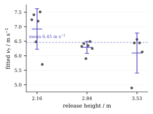
One drop is a genuine outlier: $\mathrm{𝟐}\mathbf{\%}$ on the mean.

The drop marked ^† in Table 4 has residual $3.40{\mathrm{m}}^2{\mathrm{s}}^{-2}$, over twice the median $1.34{\mathrm{m}}^2{\mathrm{s}}^{-2}$, and returns $v_{\mathrm{T}}=4.89\mathrm{m}{\mathrm{s}}^{-1}$, far below every other. Its track starts faster than a release from rest allows, so it was pushed — hard enough that the early frames are not in free flight, the one case the offset argument cannot rescue. Dropping it moves the result from $(6.45\pm 0.65)\mathrm{m}{\mathrm{s}}^{-1}$ to $(6.55\pm 0.52)\mathrm{m}{\mathrm{s}}^{-1}$, well inside the uncertainty; it is retained because the exclusion criteria were fixed before fitting and it meets them. Its real effect is on precision, inflating the standard deviation by about $30\%$.

The shuttle rotates as it falls: $\mathrm{𝟐}$–$\mathrm{𝟑}\mathbf{\%}$.

The tracked centroid is of a silhouette that changes shape as the shuttle oscillates after release, putting a wandering error of order the shuttle’s own size into $s$ — which is why $\mathrm{\Delta }s$ is $2\mathrm{cm}$ and not the $2\mathrm{mm}$ the pixel resolution alone would suggest. It is largely random between frames, so the wide gradient window suppresses it, but any persistent tilt also changes $A$ and hence $v_{\mathrm{T}}$ itself.

The fourth marker is assumed, not measured: under $\mathrm{𝟏}\mathbf{\%}$.

The lowest marker was placed at an intended $1.000\mathrm{m}$ rather than surveyed. If it is off by a centimetre, Equation 14 absorbs part of the error into $\alpha$, $\beta$, $\gamma$ and distorts the lower part of the mapping. The $1.7\mathrm{cm}$ worst residual bounds the damage, and $v_{\mathrm{T}}\propto \sqrt{\text{length}}$ halves any fractional scale error, so this stays under $1\%$ — but it is the one length in the experiment not taken with the tape.

The fall is too short to reach $v_{\mathrm{T}}$: a limit on scope.

The fastest point is about $0.8v_{\mathrm{T}}$, so the plateau in Figure 1 is extrapolated. $v_{\mathrm{T}}$ and the curve’s shape are therefore partly degenerate: a slightly different functional form with a slightly different asymptote would fit the measured range nearly as well, which is why the residual structure rather than the fitted value carries the argument.

4.1 Improvements

• Drop far enough to see the plateau. A stairwell giving $8\mathrm{m}$ would reach $0.95v_{\mathrm{T}}$, where $v^2$ visibly flattens, so $v_{\mathrm{T}}$ could be read off the graph as an asymptote instead of extrapolated. That removes the degeneracy above and would settle $v$ versus $v^2$ outright, since the two drag laws approach their plateaus at measurably different rates.

• Separate speed from fall distance. The height drift is the most interesting feature in the data and this design cannot resolve it, because a taller drop is also a faster one. Releasing from one height with a controlled initial speed, from a short vertical launcher, would vary the speed range independently of the fall distance.

• Track a fixed mark, not the silhouette. A small high-contrast mark on the cork stays put through any rotation, cutting $\mathrm{\Delta }s$ from $2\mathrm{cm}$ towards the pixel limit and directly addressing the wobble term above.